 Sign-up for free online course on ANSYS simulations!
| Include Page | ||||
|---|---|---|---|---|
|
| Include Page | ||||
|---|---|---|---|---|
|
Pre-Analysis & Start-Up
Pre-Analysis
Mathematical Model
Governing Equations
The governing equations are the continuity and Navier-Stokes equations. These equations are written in a frame of reference rotating with the blade. This has the advantage of making our simulation not require a moving mesh to account for the rotation of the blade.
The equations that we will use look as follows:
Conservation of mass:
| Wiki Markup |
|---|
{latex}
\begin{equation*}
\frac{\partial \rho}{\partial t}+\nabla \cdot \rho \vec{v}^{\,}_r =0
\end{equation*}
{latex} |
Conservation of Momentum (Navier-Stokes):
| Wiki Markup |
|---|
{latex}
\begin{equation*}
\nabla \cdot (\rho \vec{v}^{\,}_r \vec{v}^{\,}_r)+\rho(2 \vec{\omega}^{\,} \times \vec{v}^{\,}_r+\vec{\omega}^{\,} \times \vec{\omega}^{\,} \times \vec{r}^{\,})=-\nabla p +\nabla \cdot \overline{\overline{\tau}}_r
\end{equation*}
{latex} |
Where
| Wiki Markup |
|---|
{latex}$\vec{v}^{\,}_r${latex} |
| Wiki Markup |
|---|
{latex}$\vec{\omega}^{\,}${latex} |
Note the additional terms for the Coriolis force (
| Wiki Markup |
|---|
{latex}$2 \vec{\omega}^{\,} \times \vec{v}^{\,}_r${latex} |
| Wiki Markup |
|---|
{latex}$\vec{\omega}^{\,} \times \vec{\omega}^{\,} \times \vec{r}^{\,}${latex} |
| Wiki Markup |
|---|
{latex}$\vec{\omega}^{\,}= -2.22 \mathbf{\hat{k}}${latex} |
For more information about flows in a moving frame of reference, visit ANSYS Help View > Fluent > Theory Guide > 2. Flow in a Moving Frame of Reference and ANSYS Help Viewer > Fluent > User's Guide > 9. Modeling Flows with Moving Reference Frames.
Important: We use the Reynolds Averaged form of continuity and momentum and use the SST k-omega turbulence model to close the equation set.
Boundary Conditions
We model only 1/3 of the full domain using periodicity assumptions:
| Wiki Markup |
|---|
{latex}
\begin{equation*}
\vec{v}^{\,}(r_1,\theta) = \vec{v}^{\,}(r_1,\theta_1 - 120n)
\end{equation*}
{latex} |
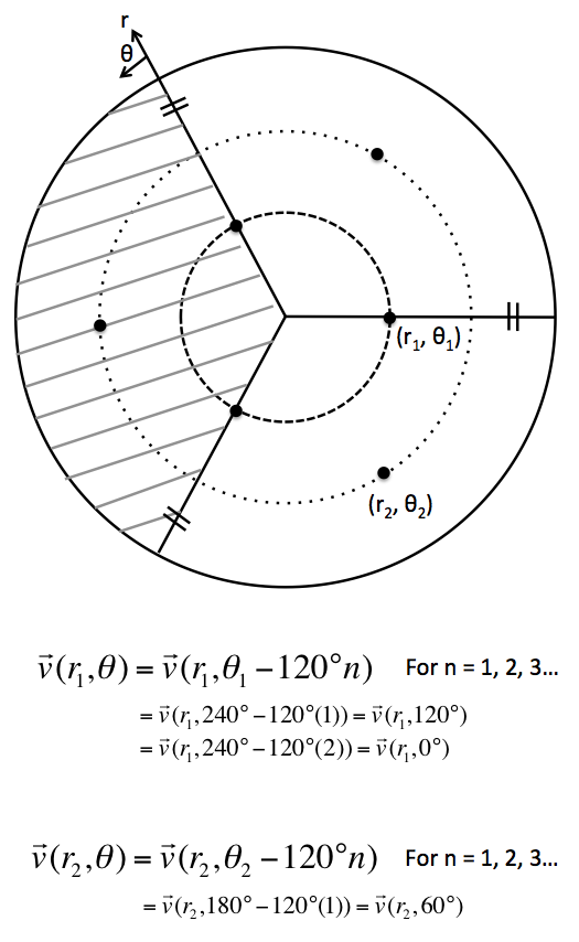
This therefore proves that the velocity distribution at theta of 0 and 120 degrees are the same. If we denote theta_1 to represent one of the periodic boundaries for the 1/3 domain and theta_2 being the other boundary, then
| Wiki Markup |
|---|
{latex}$\vec{v}^{\,}(r_i,\theta_1)=\vec{v}^{\,}(r_i,\theta_2)${latex} |
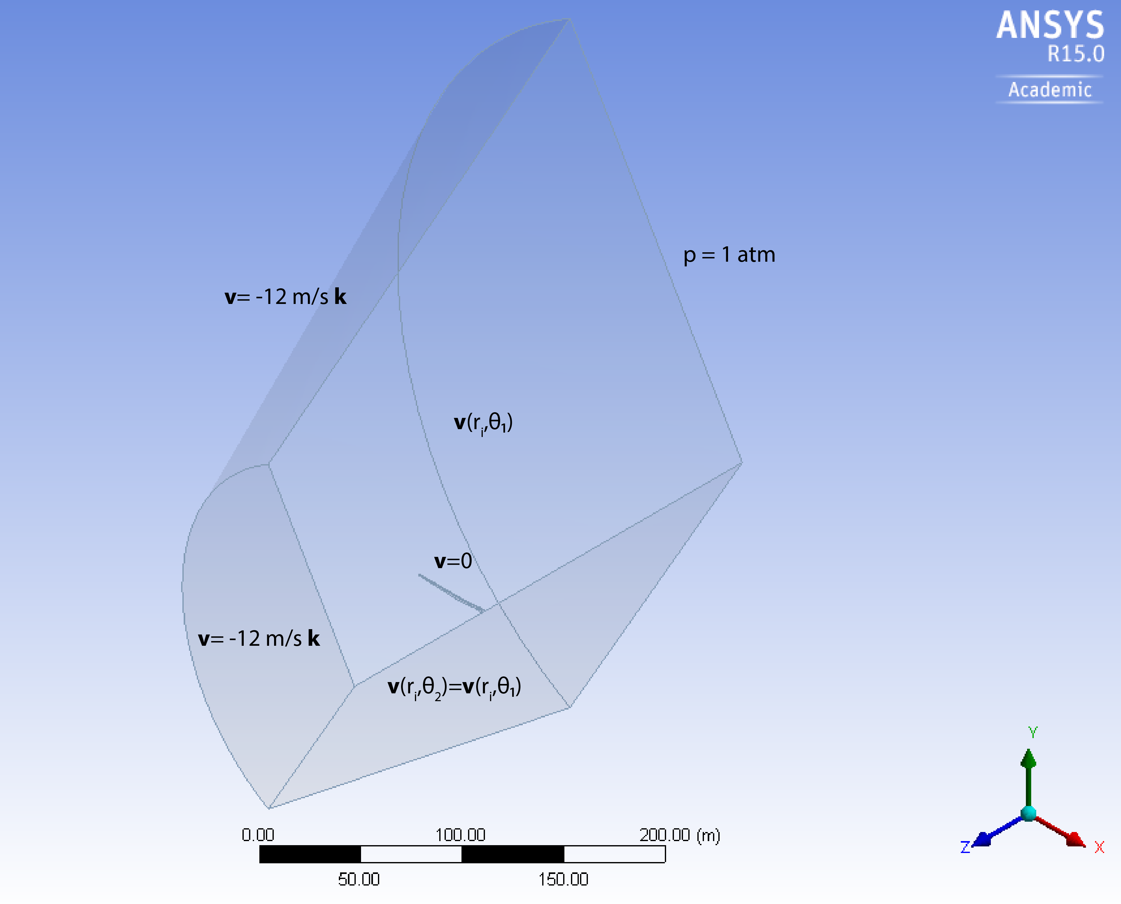
The boundary conditions on the fluid domain are as follow:
Inlet: Velocity of 12 m/s with turbulent intensity of 5% and turbulent viscosity ratio of 10
Outlet: Pressure of 1 atm
Blade: No-slip
Side Boundaries: Periodic
Numerical Solution Procedure in ANSYS
FLUENT converts these differential equations into a set of algebraic equations. Inverting these algebraic equations gives the value of (u, v, omega, p) at the cell centers. Everything else is derived from the cell centers values (post-processing). In our mesh, we'll have around 400,000 cells. The total number of unknowns and hence algebraic equations is:
400,000 * 4 = 1.6 million.
This huge set of algebraic equations is inverted through an iterative process. The matrix to be inverted is huge but sparse.
In FLUENT, we will use the pressure-based solver.
Hand-Calculations of Expected Results
One simple hand-calculation that we can do now before even starting our simulation is to find theoretical wind velocity at the tip. We can then later compare our answer with what we get from our simulation to verify that they agree.
The velocity, v, on the blade should follow the formula
| Wiki Markup |
|---|
{latex}
\begin{equation*}
v=r \times \omega_{}
\end{equation*}
{latex} |
Plugging in our angular velocity of -2.22 rad/s and using the blade length of 43.2 meters plus 1 meter to account for the distance from the root to the hub, we get
| Wiki Markup |
|---|
{latex}
\begin{equation*}
v=-2.22\ \mathrm{rad/s}\ \mathbf{\hat{k}} \times -44.2\ \mathrm{m}\ \mathbf{\hat{i}}
\end{equation*}
\begin{equation*}
v=98.1\ \mathrm{m/s}\ \mathbf{\hat{j}}
\end{equation*}
{latex} |
Start-Up
Please follow along to start this project! It is recommended to have these videos run side by side with your ANSYS project, with the video taking 1/3 of the screen space and the ANSYS window taking 2/3 of the screen space. An even better method is to use two monitors. This would allow running both the tutorial videos and ANSYS in full-screen. For example, the tutorial would be opened up on your laptop and ANSYS would be running on a lab computer. If you use the Cornell lab computers then make sure to bring some earbuds!
| HTML |
|---|
<iframe width="640" height="360" src="//www.youtube.com/embed/paSsU19hNy0" frameborder="0" allowfullscreen></iframe> |