 Sign-up for free online course on ANSYS simulations!
...
The equations that we will use look as follows:
Conservation of mass:
| Latex |
|---|
| Wiki Markup |
{latex} \begin{equation*} \frac{\partial \rho}{\partial t}+\nabla \cdot \rho \vec{v}^{\,}_r =0 \end{equation*} {latex} |
Conservation of Momentum (Navier-Stokes):
| Latex |
|---|
| Wiki Markup |
{latex} \begin{equation*} \nabla \cdot (\rho \vec{v}^{\,}_r \vec{v}^{\,}_r)+\rho(2 \vec{\omega}^{\,} \times \vec{v}^{\,}_r+\vec{\omega}^{\,} \times \vec{\omega}^{\,} \times \vec{r}^{\,})=-\nabla p +\nabla \cdot \overline{\overline{\tau}}_r \end{equation*} {latex} |
Where Wiki Markup
| Latex |
|---|
$\vec{v}^{\,}_r$ |
...
is the relative velocity (the velocity viewed from the moving frame) and Wiki Markup
| Latex |
|---|
$\vec{\omega}^{\,}$ |
...
is the angular velocity.
Note the additional terms for the Coriolis force (Wiki Markup
| Latex |
|---|
$2 \vec{\omega}^{\,} \times \vec{v}^{\,}_r$ |
...
) and the centripetal acceleration (Wiki Markup
| Latex |
|---|
$\vec{\omega}^{\,} \times \vec{\omega}^{\,} \times \vec{r}^{\,}$ |
...
) in the Navier-Stokes equations. In Fluent, we'll turn on the additional terms for a moving frame of reference and input Wiki Markup
| Latex |
|---|
$\vec{\omega}^{\,}= -2.22 \mathbf{\hat{k}}$ |
...
.
For more information about flows in a moving frame of reference, visit ANSYS Help View > Fluent > Theory Guide > 2. Flow in a Moving Frame of Reference and ANSYS Help Viewer > Fluent > User's Guide > 9. Modeling Flows with Moving Reference Frames.
...
We model only 1/3 of the full domain using periodicity assumptions:
| Latex |
|---|
| Wiki Markup |
{latex} \begin{equation*} \vec{v}^{\,}(r_1,\theta) = \vec{v}^{\,}(r_1,\theta_1 - 120n) \end{equation*} {latex} |
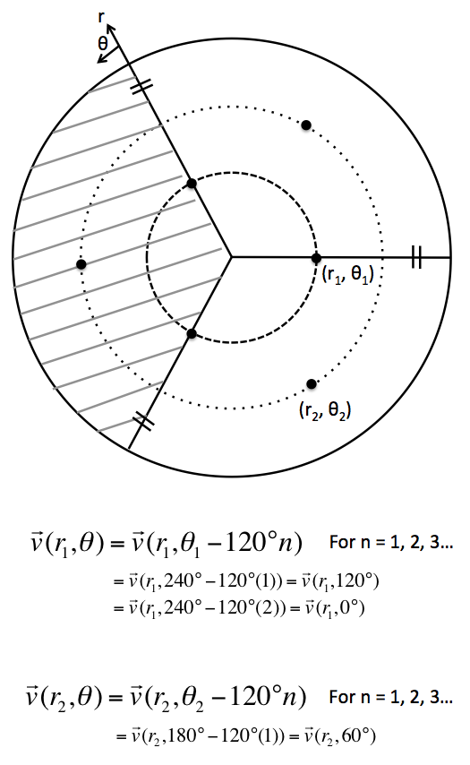
This therefore proves that the velocity distribution at theta of 0 and 120 degrees are the same. If we denote theta_1 to represent one of the periodic boundaries for the 1/3 domain and theta_2 being the other boundary, then Wiki Markup
| Latex |
|---|
$\vec{v}^{\,}(r_i,\theta_1)=\vec{v}^{\,}(r_i,\theta_2)$ |
...
.
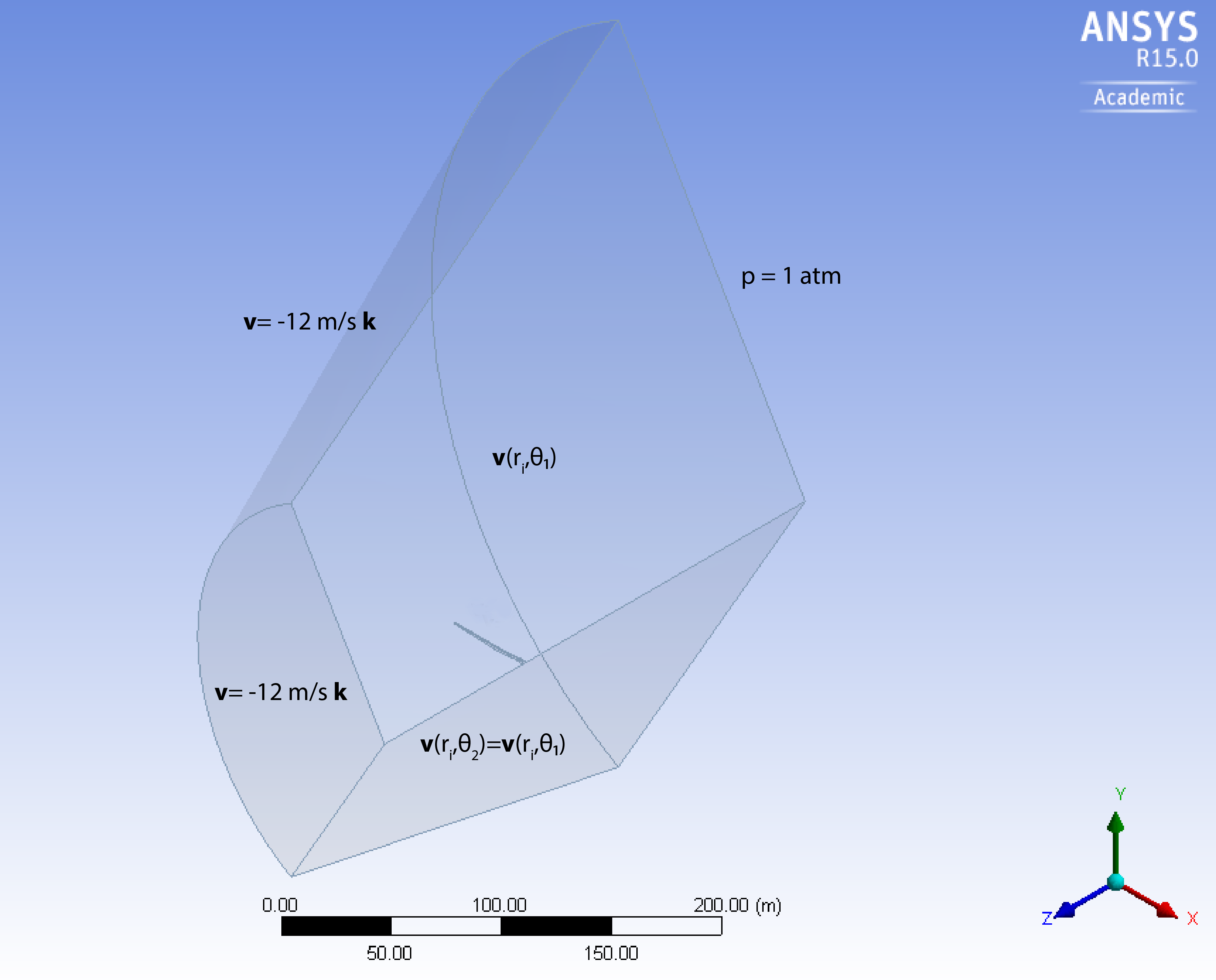
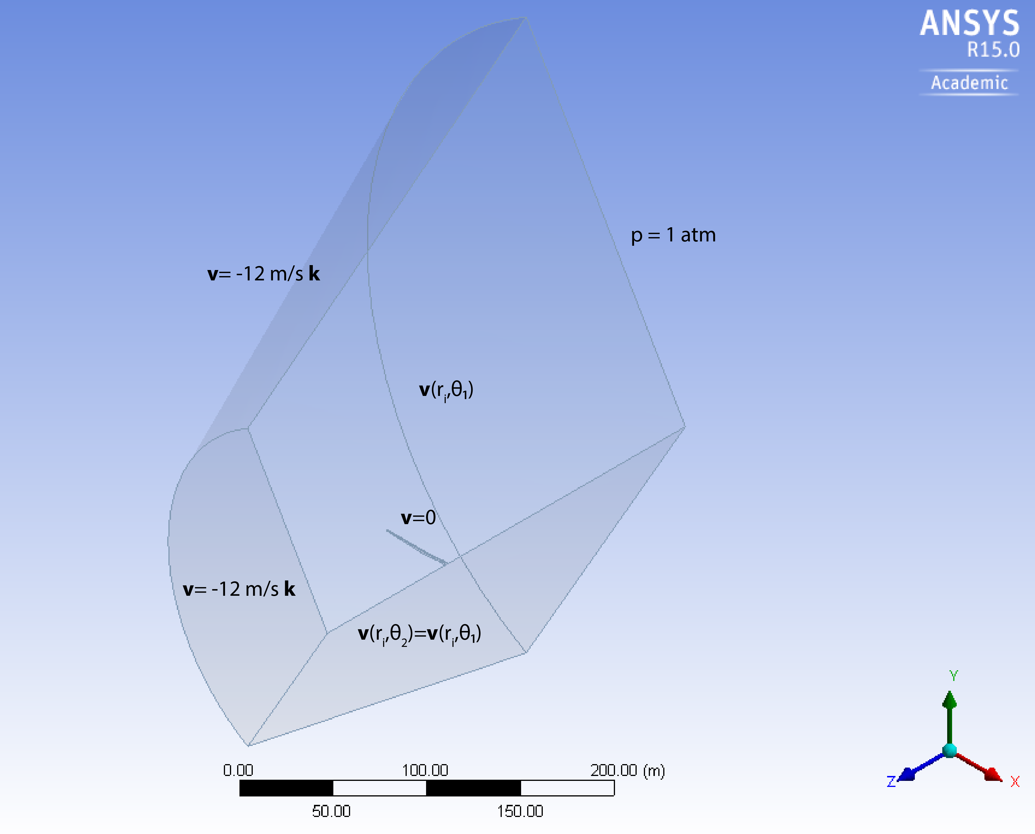
The boundary conditions on the fluid domain are as follow:
...
Side Boundaries: Periodic
Numerical Solution Procedure in ANSYS
...
The velocity, v, on the blade should follow the formula
| Latex |
|---|
| Wiki Markup |
{latex} \begin{equation*} v=r \times \omega_{} \end{equation*} {latex} |
Plugging in our angular velocity of -2.22 rad/s and using the blade length of 43.2 meters plus 1 meter to account for the distance from the root to the hub, we get
| Latex |
|---|
| Wiki Markup |
{latex} $$v=-2.22\ \mathrm{rad/s}\ \mathbf{\hat{k}} \times -44.2\ \mathrm{m}\ \mathbf{\hat{i}}$$ $$v=98.112\ \mathrm{m/s}\ \mathbf{\hat{j}}$$ {latex} |
Additionally, by using the simple one-dimensional momentum theory, we can We can also estimate the power coefficient which is the fraction of harnessed power to total power in the wind for the given turbine swept area. This analysis uses the following assumptions:
- The flow is steady, homogenous and incompressible.
- There is no frictional drag.
- There is an infinite number of blades.
- There is uniform thrust over the disc or rotor area.
- The wake is non-rotating.
- The static pressure far upstream and downstream of the rotor is equal to the undisturbed ambient pressure.
According to the M.Eng report presented in the problem statement, this blade is meant to ressemble GE 1.5 XLE wind turbine blade. The specification sheet of this turbine states the rated power of this turbine to be 1.5 MW, the rated wind speed to be 11.5 m/s and the rotor diameter to be 82.5 m.
Thus, at rated wind speed,
| Latex |
|---|
| Wiki Markup |
{latex} \begin{eqnarray*} C_p = \frac{P_{rated}}{P_{wind}} = \frac{P_{rated}}{0.5\rho A V_{rated}^3} = \frac{P_{rated}}{0.5(1.225\frac{kg}{m^3})(\frac{\pi(82.5m)^2}{4})(11.5\frac{m}{s})^3} = 0.30 \end{eqnarray*} {latex} |
The resulting power coefficient of 0.30 is very reasonable. We We will compare it to power coefficient obtained from the simulation in the Verification & Validation section.
...
| HTML |
|---|
<iframe width="640" height="360" src="//www.youtube.com/embed/paSsU19hNy0" frameborder="0" allowfullscreen></iframe> |
Summary of the above video:
- Open up ANSYS Workbench
- Drag Fluid Flow (Fluent) from Analysis Systems into Project Schematic
- Rename Project
- Save Project