 Sign-up for free online course on ANSYS simulations!
...
Wind Turbine Blade FSI (Part 1)
| Info |
|---|
This module is from our free online simulations course at edX.org (sign up here). The edX interface provides a better user experience and the content has been updated, so we recommend that you go through the module there rather than here. Also, you will be able to see answers to the questions embedded in the module there. |
Created using ANSYS 15.0 (also works in 14.5.7)
| Note |
|---|
This tutorial has videos. If you are in a computer lab, make sure to have head phones. |
| Info |
|---|
To access Part 2 of the tutorial, click here. |
...
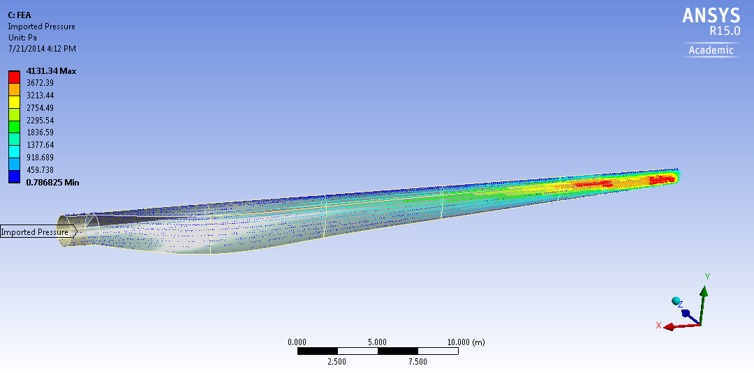
This tutorial considers the deformation due to aerodynamic loading of a wind turbine blade by performing a steady-state 1-way FSI (Fluid-Structure Interaction) analysis. Part 1 of the tutorial uses ANSYS Fluent to develop the aerodynamics loading on the blade. In part 2, the pressures on the wetted areas of the blade are passed as pressure load loads to ANSYS Mechanical to determine stresses and deformations on the blade.
The blade is 4243.3 2 meters long and starts with a cylindrical shape at the root and then transitions to the airfoils S818, S825 and S826 for the root, body and tip, respectively. This blade also has pitch to vary as a function of radius, giving it a twist and the pitch angle at the blade tip is 4 degrees. This blade was created to be similar in size to a GE 1.5XLE turbine. For more information on the dimension characteristics of this blade, please see this M.Eng report (note that model in the present tutorial has an additional 2 meter cylindrical extension at the root to make it more realistic). The
The blade is made out of an orthotropic composite material, it has a varying thickness and it also has a spar inside the blade for structural rigidity. These are further specs, which are important for the FEA simulation, are described in more detail in Part 2 of the tutorial.
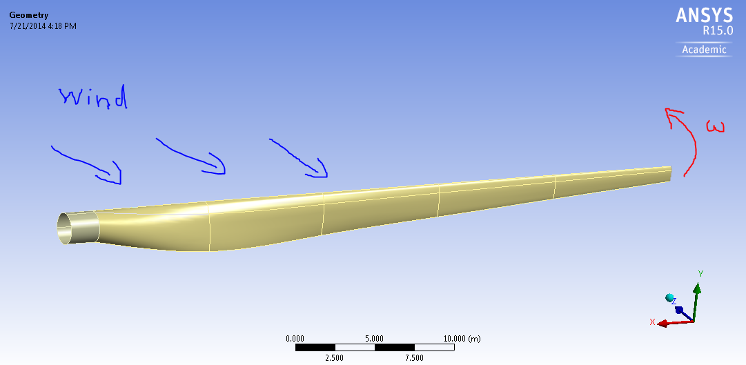
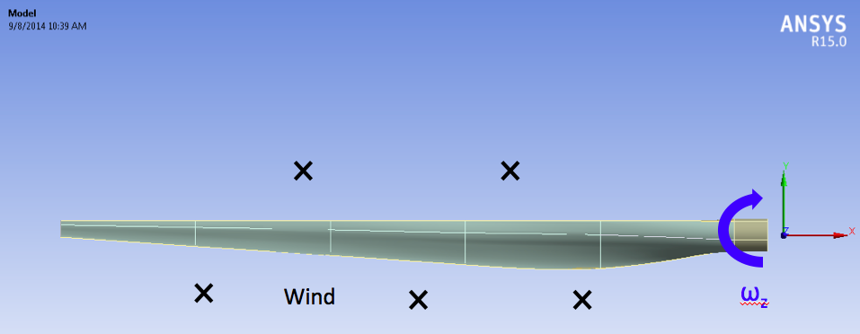
The turbulent wind flows towards the negative z-direction (into the page on the above diagram) at 12 m/s which is a typical rated wind speed for a turbine this size. This incoming flow is assumed to make the blade rotate This blade is spinning at an angular velocity of -2.22 rad/s with respect to the incoming wind from about the z-direction axis (the blade is thus spinning clockwise when looking at it from the front, like most real wind turbines). The upstream wind The tip speed (or should we say the free stream velocity?) is 12 m/s which is a typical rated wind speed for a turbine this size. (say something about it being turbulent?. This blade therefore has a tip speed ratio, which is the ratio of tip velocity to incoming wind, of 8 (also a typical value).
...
ratio (the ratio of the blade tip velocity to the incoming wind velocity) is therefore equal to 8 which is a reasonable value for a large wind turbine. Note that to represent the blade being connected to a hub, the blade root is offset from the axis of rotation by 1 meter. The hub is not included in our model.
...
Part 1
In this section of the tutorial, the blade geometry is imported, a mesh is created around the blade and the Fluent solver is then used to find the aerodynamics loading on the blade and , the fluid flow. Here is more information about the set-up.
Solver: Pressure-based
Viscous model: k-omega SST
Fluid: Air streamlines and the torque generated. We will use air at standard conditions (15 degree celcius). It's Its density is 1.225 kg/m^3 and it's its viscosity is 1.7894e-05 kg/(m*s).
Cell zone condition: Moving frame of reference (with the blade).
Main Boundary conditions:
Inlet: Velocity of 12 m/s with turbulent viscosity of 5% and turbulent viscosity ratio of 10.
Outlet: Gauge pressure of zero.
Blade: Wall
Operating conditions: Pressure at 1 atm.
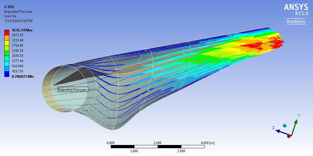
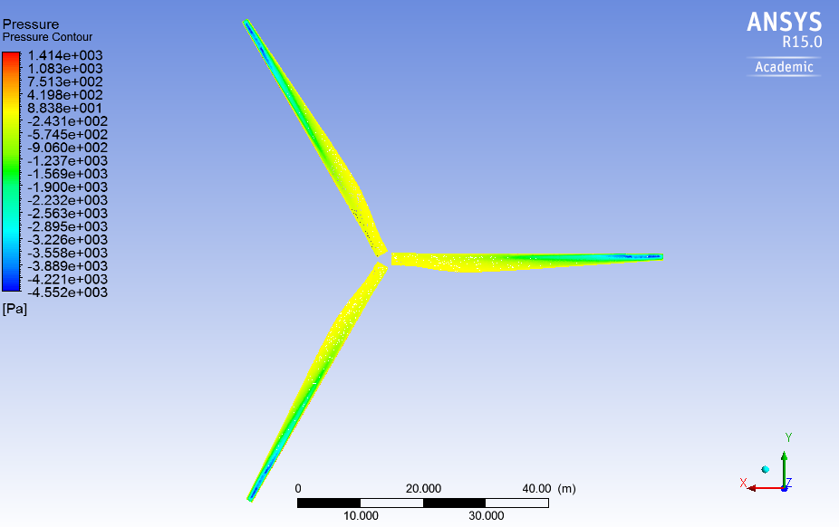
Finally, periodics are used to allow the visualization of results for three blades. Here is an example of the results that can be obtained Using periodicity, we will simulate the flow around one blade and extrapolate the solution to two more blades in order to visualize the results for a 3 blade rotor. Here's a sneak peak of a particular result that you will obtain at the end of this tutorial.
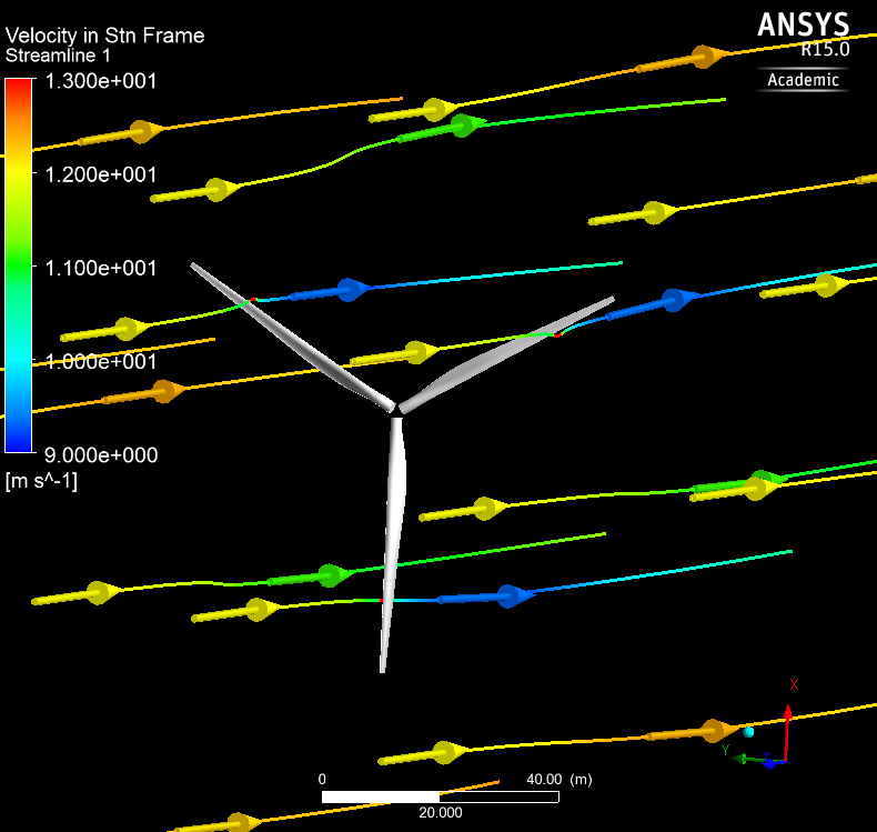
The figure is showing a pressure contour plot on the back surface of the blades.
Are you ready? Let's do this!
...
go!
Go to Step 1: Pre-Analysis & Start-Up
...