 Sign-up for free online course on ANSYS simulations!
| Include Page | ||||
|---|---|---|---|---|
|
...
| Include Page |
|---|
...
Author: John Singleton and Rajesh Bhaskaran, Cornell University
Problem Specification
1. Pre-Analysis & Start-up
2. Geometry
3. Mesh
4. Setup (Physics)
5. Solution
6. Results
7. Verification and Validation
Exercises
Discussion
|
Verification
...
& Validation
It is very important that you take the time to check the validity of your solution. This section leads you through some of the steps you can take to validate your solution.
Refine Mesh
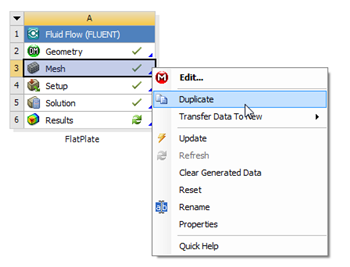
Let's repeat the solution on a finer mesh. For the finer mesh, we will increase the total number of elements(cells) by a factor of four. In order to accomplish this, we double the number of divisions on each section. Instead of modifying the project that was just created, we will duplicate it and modify the duplicate. In the Workbench Project Page right click on Mesh then click Duplicate as shown below.
| newwindow | ||||
|---|---|---|---|---|
| ||||
https://confluence.cornell.edu/download/attachments/85624049/DupMesh_Full.png |
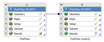
Rename the duplicate project to FlatPlate (mesh 2). You should have the following two projects in your Workbench Project Page.
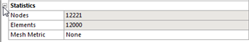
Next, double click on the Mesh cell of the FlatPlate (mesh 2) project. A new ANSYS Mesher window will open. Under Outline, expand Mesh and click on Edge Sizing. Under Details of "Edge Sizing", enter 100 for Number of Divisions. Next set the number of divisions for Edge Sizing 2 and Edge Sizing 3 to 120. Then, click Update to create the new mesh. The new mesh should now have 12000 elements (100 x 1200). A quick glance of the mesh statistics reveals that there is indeed 12000 elements.
| newwindow | ||||
|---|---|---|---|---|
| ||||
https://confluence.cornell.edu/download/attachments/141036304/MeshStat1_Full.png |
Compute the Solution
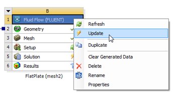
Close the ANSYS Mesher to go back to the Workbench Project Page. Under FlatPlate (mesh 2), right click on Fluid Flow (FLUENT) and click on Update, as shown below.
Now, wait a few minutes for FLUENT to obtain the solution for the refined mesh. After FLUENT obtains the solution, save your project.
Convergence
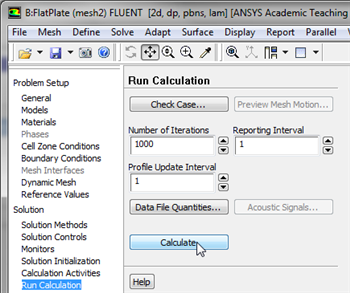
In order to launch FLUENT double click on the Solution of the "Laminar Pipe Flow (mesh 2)" project in the Workbench Project Page. The new mesh has significantly more cells, thus it is likely that the solution did not converge to the tolerances we have previously set. Therefore, we will iterate the solution further, to make sure that the solution converges. In order to do so click on Run Calculation, set Number of Iterations to 1000 and click Calculate, as shown below.
| newwindow | ||||
|---|---|---|---|---|
| ||||
https://confluence.cornell.edu/download/attachments/141036304/runcalc2_Full.png |
Once you rerun the calculation, you will quickly see that the solution did not converge for the finer mesh within 1000 iterations. The solution should converge by the 1784th iteration as shown below.

Outlet Velocity Profile
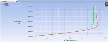
Now, the variation of the x component of the velocity will be plotted with the results of the original mesh to determine whether the solution is mesh converged. Set up a plot for the variation of the x component of the velocity along the outlet as was done in the solution section. Then load the XVelOutlet.xy file into the plot and generate the plot. You should obtain the following image.
| newwindow | ||||
|---|---|---|---|---|
| ||||
https://confluence.cornell.edu/download/attachments/141036304/VelFinal_Full.png |
As one can see from the image above, the numerical solution does not vary much at all between the two meshes. Thus, it has been confirmed that the solution is mesh converged.
Go to Exercises
Return To Problem Specification