 Sign-up for free online course on ANSYS simulations!
| Include Page | ||||
|---|---|---|---|---|
|
...
| Include Page |
|---|
...
Author: John Singleton and Rajesh Bhaskaran, Cornell University
Problem Specification
1. Pre-Analysis & Start-up
2. Geometry
3. Mesh
4. Setup (Physics)
5. Solution
6. Results
7. Verification & Validation
Exercises
Discussion
|
Numerical
...
Results
| Info | ||
|---|---|---|
| ||
We will use CFD-Post as the primary post processing GUI. Steps for post processing in FLUENT can be found here. |
Exporting Skin Friction from FLUENT into the Post-processor (CFD-Post)
FLUENT calculates the skin friction coefficient as follows (see section 34.4 of the FLUENT User's Guide which is accessible from the "help" button on the FLUENT interface).
...
Double click on Results from the Workbench Window to launch CFD-Post.
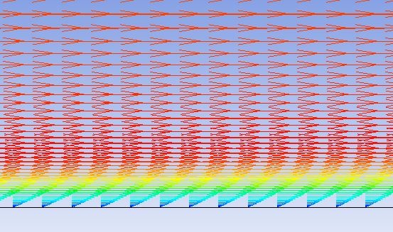
Velocity Vectors
Click on the z-axis,  to view the XY plane. Click on the vector icon to insert a vector plot. Name it Velocity Vector.
...
You can use the wheel button of the mouse to zoom into the region that closely surrounds the plate, to get a better view of the boundary layer velocities:
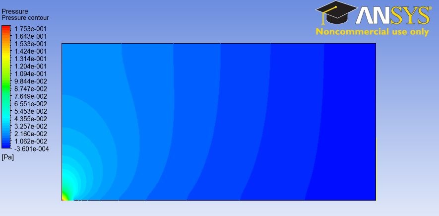
Pressure Contour
Insert > Contour. Name it Pressure contour.
...
Click on Apply to view the contour.
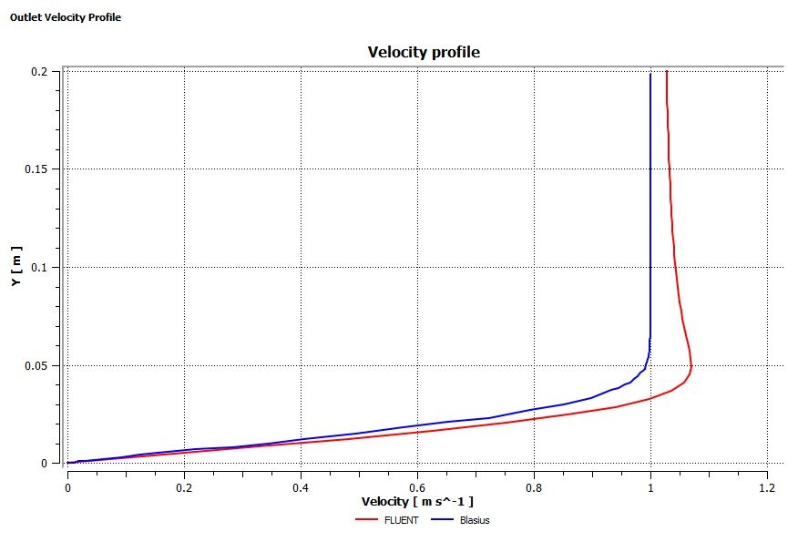
Outlet Velocity Profile
We will create a line that corresponds to the x=1 line (outlet). Then the velocity along this line can be plotted against the Y axis. From the toolbar, insert > location > line. Name it "Outlet"
...
Click on Apply. The comparison should look like the following plot:
Normalized velocity profile
We will observe the normalized velocity (u/U_infinity) at the outlet. Insert a point and call it free stream. The velocity at this point will be extracted and set to the free stream velocity (U_infinity). The velocity profile found in the previous step will be divided by U_infinity.
...
Notice the scale of this profile is exactly the same as that of the outlet velocity profile. This is because the free stream velocity, Uinf, is 1 m/s.
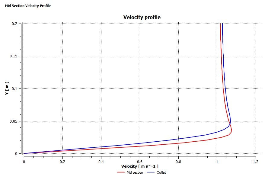
Mid-Section Velocity Profile
Here, we will plot the variation of the x component of the velocity along a vertical line in the middle of the geometry. In order to create the profile, we must first create a vertical line at x=0.5m. Insert another line, same as the previous step, and name it Mid section. Enter the following numbers to create a vertical line at x=0.5m. Set the number of samples to 50. Remember to click on Apply to finish.
...
The velocity profile comparison is shown below:
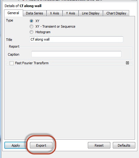
Skin Friction Coefficient
We can plot the skin friction coefficient imported from FLUENT as a function of distance along the plate. Insert a line and name it "plate wall". Enter the end points of the line and the number of samples as the following:
...
You can export the skin friction coefficient for data manipulation.
Go to Step 7: Verification & ValidationSee and rate the complete Learning Module