Pre-Analysis & Start-Up

In the Pre-Analysis step, we will review the following:

• Assumptions:  Assumptions for classical Hertz contact mechanics are discussed.
• Mathematical model:  Governing equations and boundary conditions, as well as additional relations will be discussed.
• FEM approach:  We will discuss solution strategy used in solving a nonlinear problem in FEM.

Assumptions

This problem is a classic example of Hertz Contact Mechanics*, and hence, makes the following assumptions:

...

Reference* S. Timoshenko and J.N. Goodier: "Theory “Theory of Elasticity" Elasticity” --  Chap. 13: Sect. 125, "“Pressure between Two Spherical Bodies in Contact"

Mathematical Model

As in any static analysis, the fundamental governing equations that we must keep in mind are the stress equilibrium equations (i.e. governing equation).

...

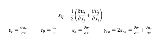
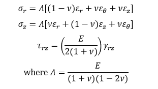
Second relationship is called Hooke's Hooke’s law.  For our model, we assume isotropic material under plane stress, and so further simplifying the Hooke's Hooke’s law results in the following equations.

FEM Approach

In this section, we discuss the general methods that ANSYS uses in solving for the desired results.  As the name suggests, finite element method first requires meshing the system that is to be analyzed into a finite number of elements.  In ANSYS, one can manually create the mesh configuration, or can alternatively let the software use a special algorithm to generate the mesh profile, which will not be discussed in this tutorial.  Depending on the level of accuracy of the results that is desirable, one can choose to refine the mesh, so that there will be more elements near any region in the model.  Having greater number of elements in the system can allow the results to converge within appropriate bounds.  It should also be noted that an element is generally comprised of multiple nodes.  Configuration of the nodes in each element can vary for different element types.  As an example, an element, PLANE183, has the configuration, as shown below.

...

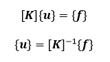
Each of the eight nodes shown above can be described by displacement vectors (translational and rotational components, depending on the element type) and by force vectors.  Finite element method first solves for the nodal displacement field with the specified boundary conditions.  The underlying system of equations that ANSYS solves for is shown below.

Wiki MarkupHere, \ [*K*\] is also referred to as the global stiffness matrix, and contains _n_ by _n_ components, where _n_ is equal to the total degrees of freedom of the system.  On the other hand, {*u*} and {*f*} are column matrices with _n_ components, which represent nodal displacement fields and nodal force fields, respectively.  After specifying the appropriate boundary condition in ANSYS, it then solves for these displacement and force fields ] is also referred to as the global stiffness matrix, and contains n by n components, where n is equal to the total degrees of freedom of the system.  On the other hand, {u} and {f} are column matrices with n components, which represent nodal displacement fields and nodal force fields, respectively.  After specifying the appropriate boundary condition in ANSYS, it then solves for these displacement and force fields simultaneously.

However, in the case of our Hertz contact example, we note that the system is a highly nonlinear problem, due to the mechanical interactions between multiple components of the system.  The fact that the boundary condition at the contact interface between the sphere and the rigid plate changes throughout the loading process indicates that an iterative approach is necessary to converge the solutions.  More specifically, we observe that the state of traction and the stiffness of the system depend on the displacement near the contact interface.

...

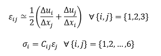
Once the solution has converged, the nodal displacement fields obtained from the final equilibrium iteration can be further used to generate the strain and stress distribution at each node.  In FEM, analyses, similar to the ones found under Mathematical Model section, are adopted to compute these nodal fields.  However, we have to modify our approach slightly to take into account the fact that we now have a finite number of elements.  This calls for a linear, first-order approximation method among the neighboring elements in computing strain distribution.  In other words, the nodal strain and stress fields are calculated in the following manner.

Start-Up

The following video shows how to create a project and set up Engineering Data for our problem. 

...

<iframe width

...

="600" height="450" src="//www.youtube.com/embed/

...

08WNUUN1c8Q?rel=0" frameborder="0" allowfullscreen></iframe>

Go to Step 2: Geometry

Go to all ANSYS Learning Modules