 Sign-up for free online course on ANSYS simulations!
| Include Page |
|---|
...
|
...
|
| Panel |
|---|
Author: John Singleton and Rajesh Bhaskaran Problem Specification |
| Include Page | ||||
|---|---|---|---|---|
|
Numerical
...
Solution
Convergence Criterion: Turn off Drag, Turn on Lift
Solution > Monitors > Drag > Edit.... Then uncheck Print to Console and uncheck Plot. Click ok.
Solution > Monitors > Lift > Edit.... Then check Print to Console, Plot and Write. Click ok. The last option writes the lift coefficient data to a file that is buried in one of the subfolders that FLUENT creates in the working folder. You'll have to dig around to find it.
If you do not see Drag or Lift under Residuals, Statistics and Force Monitors, then click on Create and select Lift (since we only want to monitor Lift right now). Then check Print to Console, Plot and Write, highlight cylinderwall and click Ok.
Solution Initialization
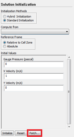
First, let's set the initial condition in all of the cells to a velocity of 1 m/s in the X-direction. Solution > Solution Initialization. Set Compute From to farfield1.. Click Initialize.
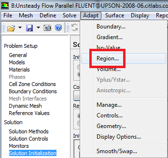
Next, we'll change the velocity in some of the cells to more quickly reach a sinusoidal variation of the lift coefficient. Adapt > Region....
Then set X Min to 0.5 m, set X Max to 32 m, set Y Min to 0 m, and set Y Max to 32m. (Note: If you instead "patch" the region 0.5 < x < 32 and -5 < y < 5, the periodic vortex shedding starts much quicker; so we recommend that).
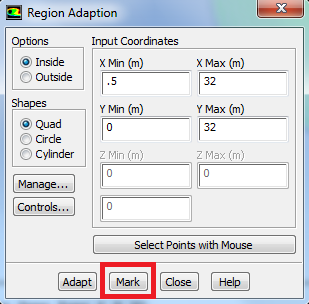
Click Mark then click Close. This will select the cells bounded by these four points, so we can change the initial condition in them.
Solution > Solution Initialization. Set Compute From to farfield1.. Click Initialize. Next, click Patch.
Complete the patching menu as shown below. This will change the initial Y component of velocity in the selected region from 0 to 0.2 m/s.
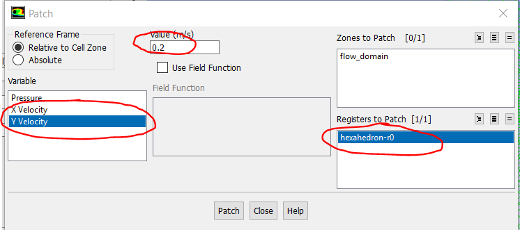
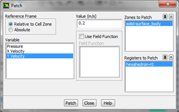
Click Patch,then click close.
View the Patch
Under Results go to Graphics and go to Contours > Setup.
Complete the set up menu as shown below:
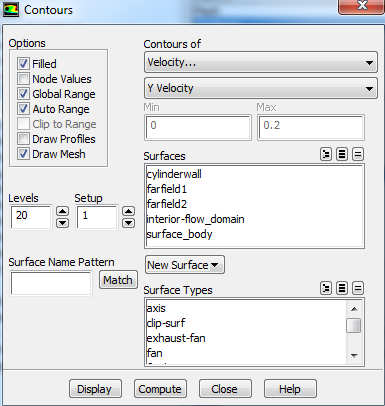
Then click Display.
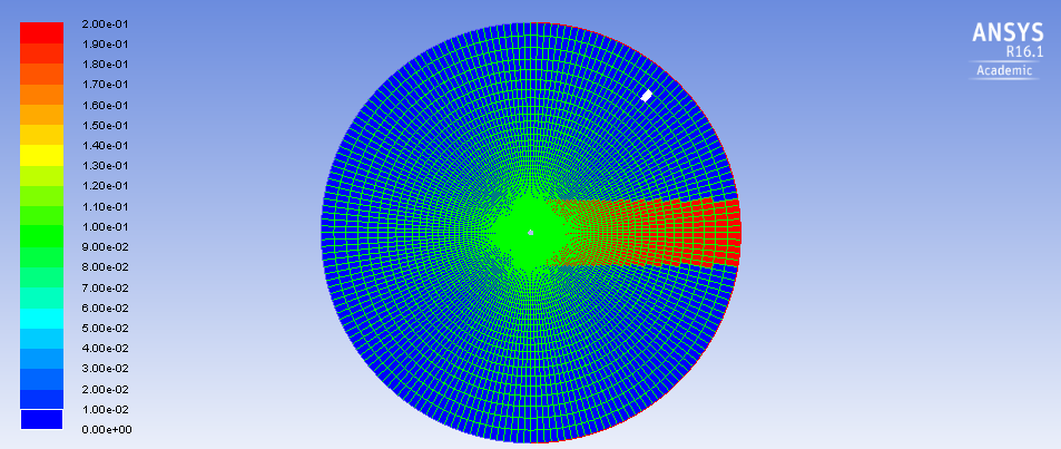
You should see the following image in the graphics window The patched region is in red, where we have changed the Y velocity to be .2 m/s to quickly induce the vortex shedding. (Note the following image is inconsistent with the settings above which perturb the initial guess only above the x axis. Sorry.)
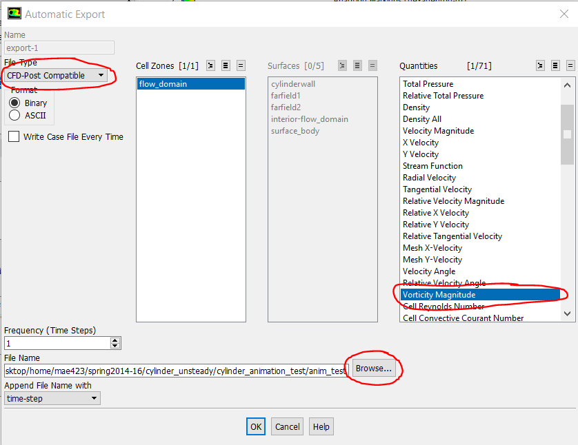
Setting Up Data Export to Create Animation
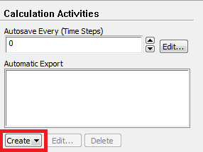
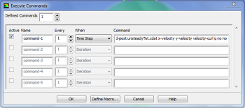
We would like to create an animation of the vorticity magnitude after the solution has been calculated. To do so, we will need to export data from FLUENT to CFD-Post, the post processor used to view results. To do so, go to {_}Solution > Calculation Activities > Execute Commands Automatic Export > Create /Edit. Now, set up the window to appear as the image below. The command entered is 'file export-to-cfd-post unsteady-%t.cdat x-velocity y-velocity velocity-curl q no no'. In this case, we will export the x and y components as well as the curl of the velocity every time step.> Solution Data Export....
Next, change File Type to CFD-Post compatible, as this is the program we will use for post processing. Then, select Vorticity Magnitude from the list of variables on the right, so we can make an animation of contours of vorticity. Finally, click Browse, and choose a convenient file location on your local drive to save the data files. Do NOT choose a folder on a flash drive as that has slow data input/output and can also cause Fluent to crash. Make note of this location for later use.
Advance Solution in Time
Solution > Run Calculation. Set Time Step Size to 0.2 seconds and set the Number Of Time Steps to 200400.
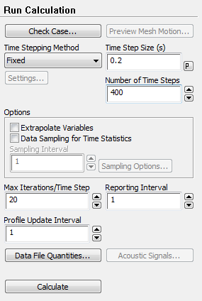
Now, click Calculate. (You may have to hit Calculate twice.) Now, have a cup of coffee. Continue the time-stepping until you get sinusoidal variation in the lift coefficientWhen complete, close FLUENT to return to the main project window.
Save Project
Go to Step 6: Results
See and rate the complete Learning ModuleNumerical Results