 Sign-up for free online course on ANSYS simulations!
...
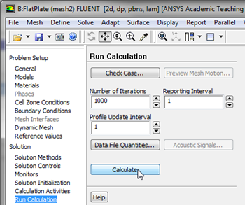
In order to launch FLUENT double click on the Solution of the "Laminar Pipe Flow (mesh 2)" project in the Workbench Project Page. The new mesh has significantly more cells, thus it is likely that the solution did not converge to the tolerances we have previously set. Therefore, we will iterate the solution further, to make sure that the solution converges. In order to do so click on Run Calculation, set Number of Iterations to 1000 and click Calculate, as shown below.
| newwindow | ||||
|---|---|---|---|---|
| ||||
https://confluence.cornell.edu/download/attachments/141036304/runcalc2_Full.png |
Once you rerun the calculation, you will quickly see that the solution did not converge for the finer mesh within 1000 iterations. The solution should converge by the 1784th iteration as shown below.

Velocity
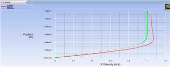
Now, the variation of the x component of the velocity will be plotted with the results of the original mesh to determine whether the solution is mesh converged. Set up a plot for the variation of the x component of the velocity along the outlet as was done in the solution section. Then load the XVelOutlet.xy file into the plot and generate the plot. You should obtain the following image.
 After, FLUENT launches (Click) Plots > XY Plot > SetUp... as shown in the image below.
For this graph, the y axis of the graph will have to be set to the y axis of the pipe (radial direction). To plot the position variable on the y axis of the graph, uncheck Position on X Axis under Options and choose Position on Y Axis instead. To make the position variable the radial distance from the centerline, under Plot Direction, change X to 0 and Y to 1. To plot the axial velocity on the x axis of the graph, select Velocity... for the first box underneath X Axis Function, and select Axial Velocity for the second box. Next, select outlet, which is located under Surfaces. Then, uncheck the Write to File check box under Options, so the graph will plot. Now, your Solution XY Plot menu should look exactly like the following image.
newwindow
https://confluence.cornell.edu/download/attachments/85624049/Solu13_Full.png| newwindow | ||||
|---|---|---|---|---|
| ||||
https://confluence.cornell.edu/download/attachments/85624049141036304/Plot2LVelFinal_Full.png |
Further Verification
The plot below shows the results of a further refined mesh ( 20 radial x 100 axial ) and the theoretical results.
newwindow
https://confluence.cornell.edu/download/attachments/85624049/PlotL_Full.png