 Sign-up for free online course on ANSYS simulations!
...
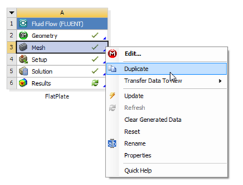
Let's repeat the solution on a finer mesh. For the finer mesh, we will use increase the total number of elements(cells) by a factor of two. In order to accomplish this, we double the number of divisions on each section. In the Workbench Project Page right click on Mesh then click Duplicate as shown below.
| newwindow | ||||
|---|---|---|---|---|
| ||||
https://confluence.cornell.edu/download/attachments/85624049/DupMesh_Full.png |
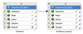
Rename the duplicate project to Laminar Pipe Flow {FlatPlate (mesh 2). You should have the following two projects in your Workbench Project Page.
Next, double click on the Mesh cell of the Laminar Pipe Flow FlatPlate (mesh 2) project. A new ANSYS Mesher window will open. Under Outline, expand Mesh and click on Edge Sizing, as shown below.
Under Details of "Edge Sizing", enter 10 for Number of Divisions, as shown below.
| newwindow | ||||
|---|---|---|---|---|
| ||||
https://confluence.cornell.edu/download/attachments/85624049/10DivSet_Full.png |
Then, click Update to generate the new mesh.
The mesh should now have 1000 elements (10 x 100). A quick glance of the mesh statistics reveals that there is indeed 1000 elements.
| newwindow | ||||
|---|---|---|---|---|
| ||||
https://confluence.cornell.edu/download/attachments/85624049/DetMesh2_Full.png |
...
Close the ANSYS Mesher to go back to the Workbench Project Page. Under Laminar Pipe Flow (mesh 2), right click on Fluid Flow (FLUENT) and click on Update, as shown below.
| newwindow | ||||
|---|---|---|---|---|
| ||||
https://confluence.cornell.edu/download/attachments/85624049/UpdateMesh2_Full.png |
Now, wait a few minutes for FLUENT to obtain the solution for the refined mesh. After FLUENT obtains the solution, save your project.
...
In order to launch FLUENT double click on the Solution of the "Laminar Pipe Flow (mesh 2)" project in the Workbench Project Page. After, FLUENT launches (Click) Plots > XY Plot > SetUp... as shown in the image below.
For this graph, the y axis of the graph will have to be set to the y axis of the pipe (radial direction). To plot the position variable on the y axis of the graph, uncheck Position on X Axis under Options and choose Position on Y Axis instead. To make the position variable the radial distance from the centerline, under Plot Direction, change X to 0 and Y to 1. To plot the axial velocity on the x axis of the graph, select Velocity... for the first box underneath X Axis Function, and select Axial Velocity for the second box. Next, select outlet, which is located under Surfaces. Then, uncheck the Write to File check box under Options, so the graph will plot. Now, your Solution XY Plot menu should look exactly like the following image.
| newwindow | ||||
|---|---|---|---|---|
| ||||
https://confluence.cornell.edu/download/attachments/85624049/Solu13_Full.png |
Since we would like to see how the results compare to the courser mesh and the theoretical solution, we will load the profile.xy file, which was created in the previous step. In order to do so, click Load File... in the Solution XY Plot menu, then select the profile.xy file. Click OK, then click Plot in the Solution XY Plot menu. You should then obtain the following plot.
| newwindow | ||||
|---|---|---|---|---|
| ||||
https://confluence.cornell.edu/download/attachments/85624049/Plot2L_Full.png |
In the plot above the green dots correspond to the theoretical solution, the red dots correspond to the rough mesh ( 5 x 100 ), and the white dots correspond to the refined mesh ( 10 x 100 ). Note how the refined mesh results resemble the theory signicantly more than the rough mesh.
...
The plot below shows the results of a further refined mesh ( 20 radial x 100 axial ) and the theoretical results.
| newwindow | ||||
|---|---|---|---|---|
| ||||
https://confluence.cornell.edu/download/attachments/85624049/PlotL_Full.png |
Notice that for the further refined mesh, the results are almost indistinguishable from theory.