Page History

Panel
Author: John Singleton and Rajesh Bhaskaran, Cornell University Problem Specification 1. Pre-Analysis & Start-up 2. Geometry 3. Mesh 4. Setup (Physics) 5. Solution 6. Results 7. Verification & Validation

Note
title Under Construction
This page of this tutorial is currently under construction. Please check back soon.

Info
title Useful Information
Click here for the FLUENT 6.3 version.

Step 6: Results

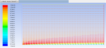
Velocity Vectors

One can plot vectors in the entire domain, or on selected surfaces. Here, the vectors will be plotted for the entire domain. First, click on Graphics & Animations . Next, double click on Vectors which is located under Graphics. Then, click on Display in the Vectors menu. You should obtain, the following output.

newwindow
Higher Resolution Image Higher Resolution Image
https://confluence.cornell.edu/download/attachments/118771111/VectPlot_Full.png

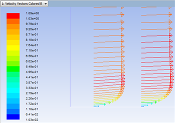
You can use the wheel button of the mouse to zoom into the region that closely surrounds the plate, to get a better view of the boundary layer velocities.

newwindow
Higher Resolution Image Higher Resolution Image
https://confluence.cornell.edu/download/attachments/118771111/VectPlot2_Full.png

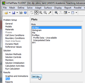
Outlet Velocity Profile

In this section we will first plot the variation of the x component of the velocity along the outlet. Then we will plot the Blasius solution to see how the numerical solution compares. In order to start the process (Click) Results > Plots > XY Plot... > Set Up.. as shown below.

newwindow
Higher Resolution Image Higher Resolution Image
https://confluence.cornell.edu/download/attachments/118771111/xyplotsetup_Full.png

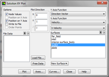
In the Solution XY Plot menu make sure that Position on Y Axis is selected , and X is set to 0 and Y is set to 1. This tells FLUENT to plot the y-coordinate value on the ordinate of the graph. Next, select Velocity... for the first box underneath X Axis Function and select X Velocity for the second box. Please note that X Axis Function and Y Axis Function describe the x and y axes of the graph, which should not be confused with the x and y directions of the geometry. Finally, select outlet under Surfaces since we are plotting the x component of the velocity along the outlet. This finishes setting up the plotting parameters. Your Solution XY Plot menu should look exactly the same as the following image.

newwindow
Higher Resolution Image Higher Resolution Image
https://confluence.cornell.edu/download/attachments/118771111/SolXY1_Full.png

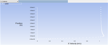
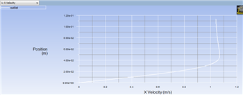
Now, click Plot. The plot of the x component of the velocity as a function of distance along the outlet now appears.

newwindow
Higher Resolution Image Higher Resolution Image
https://confluence.cornell.edu/download/attachments/118771111/XVelPlot1_Full.png

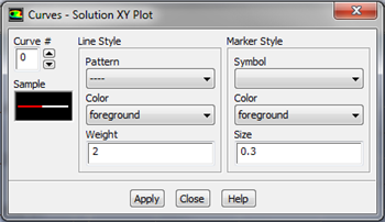
In order to increase the legibility of the graph, we will plot the data as a line rather than points. To turn on the line feature, click on Curves... in the Solution XY Plot menu. Then, set Pattern to ----, set the Weight to 2 and select nothing for Symbol, as shown below.

newwindow
Higher Resolution Image Higher Resolution Image
https://confluence.cornell.edu/download/attachments/118771111/Curv2_Full.png

Next, click Apply in the Curves - Solution XY Plot menu. Next, close the Curves - Solution XY Plot menu.

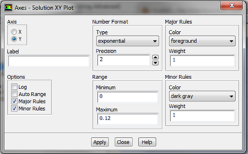
Now, the range of the y axis will be truncated, as we are not interested in far field velocity. Furthermore, the grid lines will be turned on. In order to implement these two changes. First click Axes in the Solution XY Plot menu. Next, select Y for Axis, deselect Auto Range, select Major Rules, select Minor Rules. Then, set Minimum to 0 and set Maximum to 0.12. Your Axes - Solution XY Plot menu, should look exactly like the image below.

newwindow
Higher Resolution Image Higher Resolution Image
https://confluence.cornell.edu/download/attachments/118771111/AxesMen1_Full.png

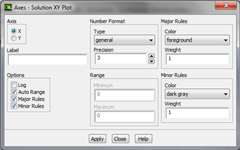
Then, click Apply in the Axes - Solution XY Plot menu. Now, select X for Axis and select Major Rules and Minor Rules, as shown below.

newwindow
Higher Resolution Image Higher Resolution Image
https://confluence.cornell.edu/download/attachments/118771111/Axes2_Full.png

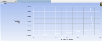
Next, click Apply in the Axes - Solution XY Plot menu. Close the Axes - Solution XY Plot menu. Now, click Plot menu in the Solution XY Plot menu. You should obtain the following output.

newwindow
Higher Resolution Image Higher Resolution Image
https://confluence.cornell.edu/download/attachments/118771111/Plot5_Full.png

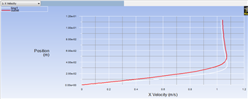
It is of interest to compare the numerical velocity profile to the velocity profile obtained from the Blasius solution. In order to plot the theoretical results, first click here to download the necessary file. Save the file to your working directory. Next, go to the Solution XY Plot menu and click Load File... and select the file that you just downloaded, BlasiusU.xy. Lastly, click Plot in the Solution XY Plot menu. You should then obtain the following figure.

newwindow
Higher Resolution Image Higher Resolution Image
https://confluence.cornell.edu/download/attachments/118771111/Plot6_Full.png

Lastly, select Write to File located under Options in the Solution XY Plot menu. Then, click Write.... When prompted for a filename, enter XVelOutlet.xy and save the file in your working directory.

Mid-Section Velocity Profile

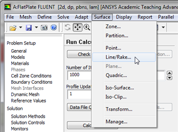
Here, we will plot the variation of the x component of the velocity along a vertical line in the middle of the geometry. In order to create the profile, we must first create a vertical line at x=0.5m, using the Line/Rake tool. First, (Click) Surface < Line/Rake as shown in the following image.

newwindow
Higher Resolution Image Higher Resolution Image
https://confluence.cornell.edu/download/attachments/118771111/SurfLinRake_Full.png

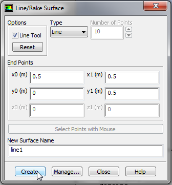
We'll create a straight vertical line from (x0,y0)=(0.5,0) to (x1,y1)=(0.5,0.5). Select Line Tool under Options. Enter x0=0.5, y0=0,x1=0.5, y1=0.5. Enter line1 under New Surface Name. Your Line/Rake Surface menu should look exactly like the following image. Then, click Create.



Next, click Create. Now, that the vertical line has been created we can proceed to the plotting. Click on Plots, then double click XY Plot to open the Solution XY Plot menu. In the Solution XY Plot menu, use the settings that were used from the section above, except select line1 under Surfaces and deselect any other geometry sections. Make sure that Write to File is not selected, then click Plot. You should obtain the following output.

newwindow
Higher Resolution Image Higher Resolution Image
https://confluence.cornell.edu/download/attachments/118771111/Plot1M_Full.png

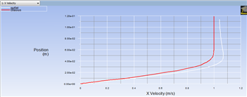
Then, return to the Solution XY Plot menu and select both line1 and outlet under Surfaces. Next, click Plot and you should obtain the following figure.

newwindow
Higher Resolution Image Higher Resolution Image
https://confluence.cornell.edu/download/attachments/118771111/Plot2M_Full.png

Once again, return to the Solution XY Plot menu, select Write to File, then click Write.... When prompted for a filename, enter XVelProfs.xy and save the file in your working directory.

Pressure Coefficients

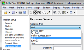
In this section we will create contour plots for the pressure coefficients. Before we begin, we must first set the reference values for velocity. In order to do so, first click on Reference Values then set Compute from to inlet, as shown below.

newwindow
Higher Resolution Image Higher Resolution Image
https://confluence.cornell.edu/download/attachments/118771111/CompInlet_Full.png

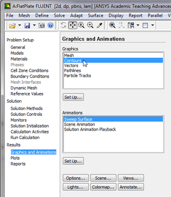
Next, click on Graphics and Animations, then double click on Contours, as shown below.

newwindow
Higher Resolution Image Higher Resolution Image
https://confluence.cornell.edu/download/attachments/118771111/ContPlot_Full.png

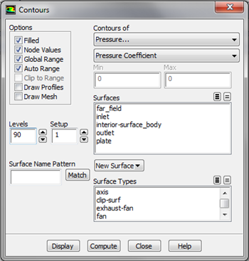
In the Contours menu, set Contours of to Pressure... and set the box below to Pressure Coefficient. Next, select Filled and set Levels to 90. Your Contours menu should look exactly like the following image.

newwindow
Higher Resolution Image Higher Resolution Image
https://confluence.cornell.edu/download/attachments/118771111/Contou_Full.png

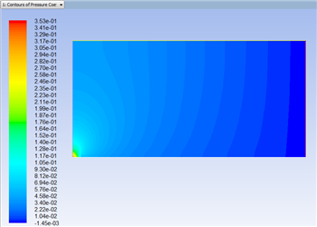
Lastly, click Display in the Contours menu to generate the contour plot. You should obtain the following output.

newwindow
Higher Resolution Image Higher Resolution Image
https://confluence.cornell.edu/download/attachments/118771111/ContP1_Full.png

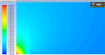
You can then zoom in to the leading edge of the plate with the wheel mouse button as shown below.

newwindow
Higher Resolution Image Higher Resolution Image
https://confluence.cornell.edu/download/attachments/118771111/ContZoom_Full.png

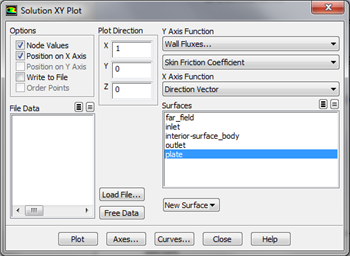
Skin Friction Coefficient

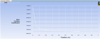
Here, the skin friction coefficient will be plotted as a function of distance along the plate. First, click on Plots, then double click on XY Plot. In the Solution XY Plot menu deselect Write to File, select Position on X Axis, set X to 1 and set Y to 0. Then, set the box located underneath Y Axis Function to Wall Fluxes and set the box below to Skin Friction Coefficient. Next, select plate under Surfaces and deselect any other geometry features. At this point your Solution XY Plot menu should look the same as the following image.

newwindow
Higher Resolution Image Higher Resolution Image
https://confluence.cornell.edu/download/attachments/118771111/SolXY3_Full.png

Make sure that for both the x and y axes, that Auto Range is selected. Remember, that you must click Apply to implement the changes you make. Then, click Plot in the Solution XY Plot menu and you should obtain the following output.

newwindow
Higher Resolution Image Higher Resolution Image
https://confluence.cornell.edu/download/attachments/118771111/SkinFric1_Full.png

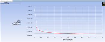
It is of interest to compare the numerical skin friction coefficient profile to the skin friction coefficient profile obtained from the Blasius solution. In order to plot the theoretical results, first click here to download the necessary file. Save the file to your working directory. Next, go to the Solution XY Plot menu and click Load File... and select the file that you just downloaded, BlasiusSkin.xy. Lastly, click Plot in the Solution XY Plot menu. You should then obtain the following figure.

newwindow
Higher Resolution Image Higher Resolution Image
https://confluence.cornell.edu/download/attachments/118771111/SkinFric2_Full.png

Lastly, select Write to File located under Options in the Solution XY Plot menu. Then, click Write.... When prompted for a filename, enter SkinFriction.xy and save the file in your working directory.

Drag

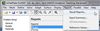
Now, we will obtain the drag on the plate. First, click on Report then click on Result Reports..., as shown in the following image.

newwindow
Higher Resolution Image Higher Resolution Image
https://confluence.cornell.edu/download/attachments/118771111/Report_RR_Full.png

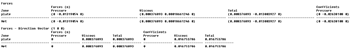
Next, double click on Forces and click Print in the Force Reports menu. You should then obtain the following output in the command pane.

newwindow
Higher Resolution Image Higher Resolution Image
https://confluence.cornell.edu/download/attachments/118771111/ForceRep_Full.png

As one can see from the data above, the plate experiences a drag of approximately 0.008377 Newtons. Furthermore, the data states that the drag coefficient is approximately 0.01675.

Go to Step 7: Verification & Validation

See and rate the complete Learning Module

Go to all FLUENT Learning Modules