Page History

...

https://confluence.cornell.edu/download/attachments/118771111/step6_007.png?version=1

Plot Velocity Profiles

Results > Plots > XY Plot

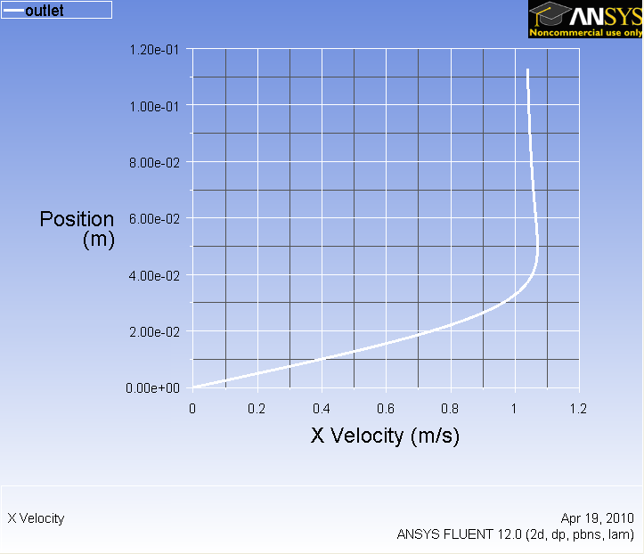
Uncheck Position on X Axis and check Position on Y Axis under Options. Under Plot Direction, set X to 0 and Y to 1. Under X Axis Function, select Velocity...Then, change Velocity Magnitude to X Velocity. Finally under surface, select outlet. Before we are ready to plot, click on the Axes... button and rescale the y-axis from 0 to 0.12. Also, check the Major Rules and Minor Rules for both axes. Remember that you must click the Apply button when performing changes in each axis.

Click Plot.
Image Removed

...

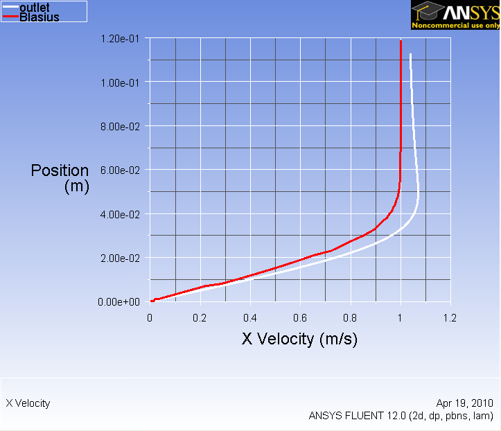
https://confluence.cornell.edu/download/attachments/118771111/step6_008.png?version=1

To compare with the Blasius solution, download the solution here. Click Load File...and select the file you just downloaded. Then plot the solutions again to display both lines on the same graph.

Image Removed

...

https://confluence.cornell.edu/download/attachments/118771111/step6_009.png?version=1

What is the noticeably different between two solutions? Why is the velocity overshoot 1 for FLUENT's solution?

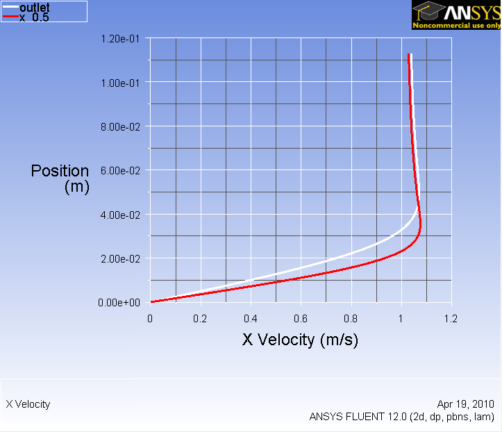
Now we will compare the velocity profile at two sections. Create another section in the middle of the plate.

Again, in the XY Plot window under New Surface > Line/Rake

Check the line tool checkbox under Options and set the initial coordinate to (0.5,0) and final coordinate to (0.5,0.5). Under the New Surface Name field, type in x_0.5 and then click the Create button to create the line.

We can now plot and compare the velocity profile at the mid point and the outlet of the flow.

Under Surfaces, select outlet and {}x_0.5 and Plot.

Image Removed

...

https://confluence.cornell.edu/download/attachments/118771111/step6_010.png?version=1

Go to Step 7: Refine Mesh