Page History

...

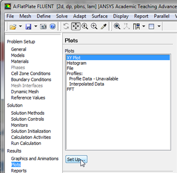
In this section we will first plot the variation of the x component of the velocity along the outlet. In order to start the process (Click) Results > Plots > XY Plot... > Set Up.. as shown below.

newwindow
Higher Resolution Image Higher Resolution Image
https://confluence.cornell.edu/download/attachments/118771111/xyplotsetup_Full.png

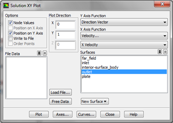
In the Solution XY Plot menu make sure that Position on Y Axis is selected , and X is set to 0 and Y is set to 1. This tells FLUENT to plot the y-coordinate value on the ordinate of the graph. Next, select Velocity... for the first box underneath X Axis Function and select X Velocity for the second box. Please note that X Axis Function and Y Axis Function describe the x and y axes of the graph, which should not be confused with the x and y directions of the geometry. Finally, select outlet under Surfaces since we are plotting the x component of the velocity along the outlet. This finishes setting up the plotting parameters. Your Solution XY Plot menu should look exactly the same as the following image.

newwindow
Higher Resolution Image Higher Resolution Image
https://confluence.cornell.edu/download/attachments/118771111/SolXY1_Full.png

Image Removed

newwindow
Higher Resolution Image	Higher Resolution Image	https://confluence.cornell.edu/download/attachments/118475269/SolutionXYPlot_Full.png

Now, click Plot. The plot of the x component of the axial velocity as a function of distance along the centerline outlet now appears.
Image Removed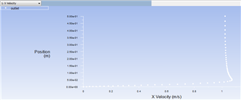
Image Added

newwindow
Higher Resolution Image Higher Resolution Image
https://confluence.cornell.edu/download/attachments/118475269118771111/Plot1CenterlineXVelPlot1_Full.png

Plot Pressure Coefficients

...