...
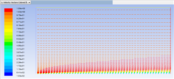
One can plot vectors in the entire domain, or on selected surfaces. Here, the vectors will be plotted for the entire domain. First, click on Graphics & Animations . Next, double click on Vectors which is located under Graphics. Then, click on Display in the Vectors menu. You should obtain, the following output.
| newwindow |
|---|
| Higher Resolution Image |
|---|
| Higher Resolution Image |
|---|
|
https://confluence.cornell.edu/download/attachments/118771111/VectPlot_Full.png |
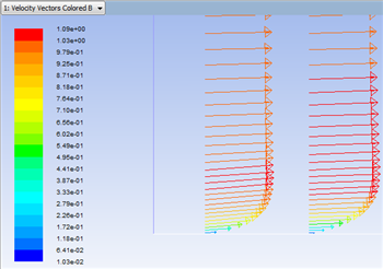
You can use the wheel button of the mouse to zoom into the region that closely surrounds the plate, to get a better view of the boundary layer velocities.
| newwindow |
|---|
| Higher Resolution Image |
|---|
| Higher Resolution Image |
|---|
|
https://confluence.cornell.edu/download/attachments/118771111/VectPlot2_Full.png |
Outlet Velocity Profile
In this section we will first plot the variation of the x component of the velocity along the outlet. In order to start the process (Click) Results > Plots > XY Plot... > Set Up.. as shown below.
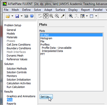 Image Added
| newwindow |
|---|
| Higher Resolution Image |
|---|
| Higher Resolution Image |
|---|
|
https://confluence.cornell.edu/download/attachments/118771111/xyplotsetup_Full.png |
In the Solution XY Plot menu make sure that Position on X Axis is selected , and X is set to 1 and Y is set to 0. This tells FLUENT to plot the x-coordinate value on the abscissa of the graph. Next, select Velocity... for the first box underneath Y Axis Function and select Axial Velocity for the second box. Please note that X Axis Function and Y Axis Function describe the x and y axes of the graph, which should not be confused with the x and y directions of the pipe. Finally, select centerline under Surfaces since we are plotting the axial velocity along the centerline. This finishes setting up the plotting parameters. Your Solution XY Plot should look exactly the same as the following image.  Image Added
| newwindow |
|---|
| Higher Resolution Image |
|---|
| Higher Resolution Image |
|---|
|
https://confluence.cornell.edu/download/attachments/118475269/SolutionXYPlot_Full.png |
Now, click Plot. The plot of the axial velocity as a function of distance along the centerline now appears. Image Added| newwindow |
|---|
| Higher Resolution Image |
|---|
| Higher Resolution Image |
|---|
|
https://confluence.cornell.edu/download/attachments/118475269/Plot1Centerline_Full.png |
Plot Pressure Coefficients
...
 Sign-up for free online course on ANSYS simulations!