 Sign-up for free online course on ANSYS simulations!
| Include Page | ||||
|---|---|---|---|---|
|
| Include Page | ||||
|---|---|---|---|---|
|
| Note |
|---|
If equations below don't display properly and you get a "latex plugin" error, please refresh the page. |
...
Assumptions
We'll assume that:
Plane stress conditions apply since the bar is thin, thus we don't expect significant variation of stresses in the z direction:
Latex \begin{align*}Wiki Markup {latex}\[ \sigma_{z} = \tau_{xz} = \tau_{yz} = 0 \] end{latexalign*}
Gravity effects can be neglected i.e. no body forces.
Latex \begin{align*}Wiki Markup {latex} \[ F_x = F_y =0 \] end{latexalign*}
Governing Equations
Since we are assuming plane stress conditions, we can use the 2D version of the equilibrium equations. When the deformed structure reaches equilibrium, the 2D stress components should satisfy the 2D equilibrium equations with zero body forces:
| Latex |
|---|
| Wiki Markup |
{latex} \begin{eqnarrayalign*} {\partial \sigma_x \over \partial x} + {\partial \tau_{xy} \over \partial y} = 0 \nonumber \\ {\partial \tau_{xy} \over \partial x} + {\partial \sigma_y \over \partial y} = 0 \nonumber \end{eqnarray} {latex}align*} |
Boundary Conditions
We solve these equations in a rectangular domain and impose the appropriate boundary conditions. At every point on the boundary, either the displacement or the traction must be prescribed.
...
The bottom and top edges are free. If a boundary location is not constrained and can move freely, it can expand and contract without incurring stress. Thus, traction on the free edges is zero and we get
get
| Latex |
|---|
\begin{align*} |
| Wiki Markup |
{latex} \[ \sigma_y = \tau_{xy} = 0 \:\: at \: y = 0 \: and \: y = H \] end{latexalign*} |
The left end is fixed. So both components of displacement are zero at this end:
| Latex |
|---|
\begin{align*}
|
| Wiki Markup |
{latex} \[ u = v = 0 \:\: at \: x = 0 \] end{latexalign*} |
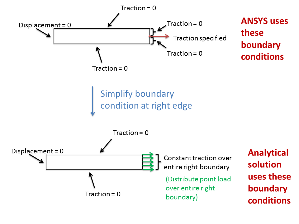
The boundary condition is a little bit more complicated at the right end. Here, the traction is specified at the mid-point where the point load is applied. The applied traction at all other points on the right boundary is zero. For brevity, we won't write out the corresponding equations at the right boundary. We'll simplify this boundary condition in our hand calculations below (to make the problem tractable) but the ANSYS solution provided uses the full set of boundary conditions. Another complication is that since we have a point load, the specified traction at the mid-point of the right end is infinite. We'll later discuss the effect of this in the ANSYS solution. Do keep in mind that there are no point loads in practice, it's just an idealization that can lead to weird behavior that we need to be aware of.
...
Additional Assumptions in Hand Calculations
We'll simplify the right boundary condition. Instead of a point load, we'll assume that the load is distributed over the entire right boundary. So the traction condition at the right boundary becomes
Latex \begin{align*Wiki Markup {latex} \[ \sigma_x = P/(H \, t), \: \: \tau_{xy} = 0 \: \: \: at \: x = L \] end{latexalign*}
Here, t is the thickness.
The following schematic shows the process of simplifying the right boundary condition in the hand calculation.
Away from the left and right ends, we expect a uni-axial state of stress with zero shear (OK, this is a bit of a leap of the imagination but it's plausible). So we'll assume that everywhere
Latex \begin{align*Wiki Markup {latex} \[ \tau_{xy} = 0 \] end{latexalign*}
We don't expect this to hold near the left boundary or in the vicinity of the point load, so our hand calculations won't be valid there.
Analytical Solution
With these additional assumptions in hand, we can easily solve the BVP and we get the following analytical solution:
| Latex |
|---|
\begin{align* |
| Wiki Markup |
{latex} \[ \sigma_x = P/(H \, t), \: \: \: \sigma_y = 0 \] end{latexalign*} |
This is the well known (P/A) result but we have arrived at it somewhat carefully, accounting for the additional assumptions we made in the process. We'll need to keep these additional assumptions in mind when comparing the hand calculations with the ANSYS solution. For the values given in the problem statement, we have
| Latex |
|---|
| Wiki Markup |
{latex} \begin{eqnarrayalign*} \sigma_x = 2000/(10*1) = 200 \ N/mm^2 = 200 \ MPa \nonumber \end{eqnarray} {latex}align*} |
The corresponding strain in the x-direction can be calculated from Hooke' law:
| Latex |
|---|
\begin{align*} |
| Wiki Markup |
{latex} \[ \epsilon_x = \frac{\sigma_x}{E} - \nu \, \frac{\sigma_y}{E} = 1 \times 10^{-6} \] end{latexalign*} |
The strain is tiny since the material is very stiff with an Young's modulus of 200 GPa. The displacement at the right end can be estimated by integrating the constant x-strain:Wiki Markup
| Latex |
|---|
\begin{align*} \ |
...
epsilon_x = \frac{\partial u}{\partial x}
\ |
...
end{ |
...
align*} |
| Latex |
|---|
\begin{align*} |
| Wiki Markup |
{latex} \[ u(x=L) = \int_0^L{\epsilon_x} \, dx = 0.05 \, mm \] end{latexalign*} |
The above hand calculations give us expected values of stress, strain and displacement which we'll compare with the ANSYS results.
...
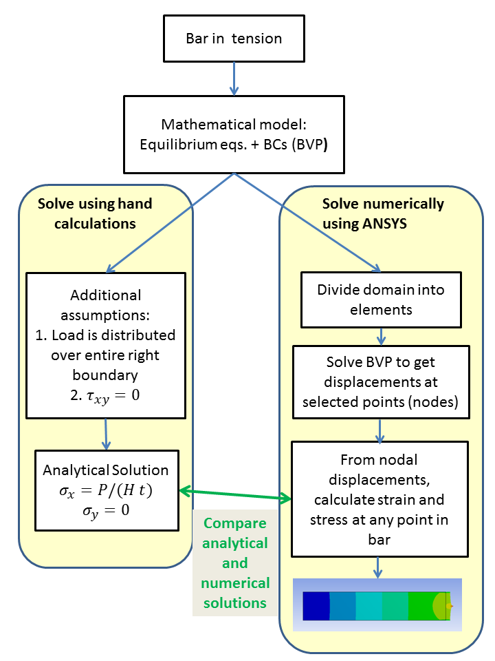
The following figure summarizes the contrasts between the hand calculations and ANSYS's approach. One important point to keep in mind is that both start with the same mathematical model but use different assumptions and approximations to solve it. Also, in FEA, one always computes the displacement first and from that derives the stress. Contrast that to the hand calculations where we calculated the stress first and from that derived the displacement. The latter process works only for a few simple problems.
This brings us to the end of the Pre-Analysis section.
...
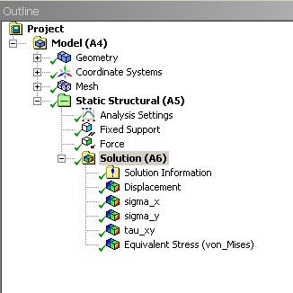
We'll investigate the items listed under Solution (A6) in the next step of this tutorial.
Go to Step 2: Numerical Results
...