FLUENT - Flat Plate Boundary Layer Step 6

...

...

...

...

...

...

...

...

Step 6: Analyze Results

Plot Velocity Vectors

...

Zoom in a little using the middle mouse button to peer more closely at the velocity vectors.
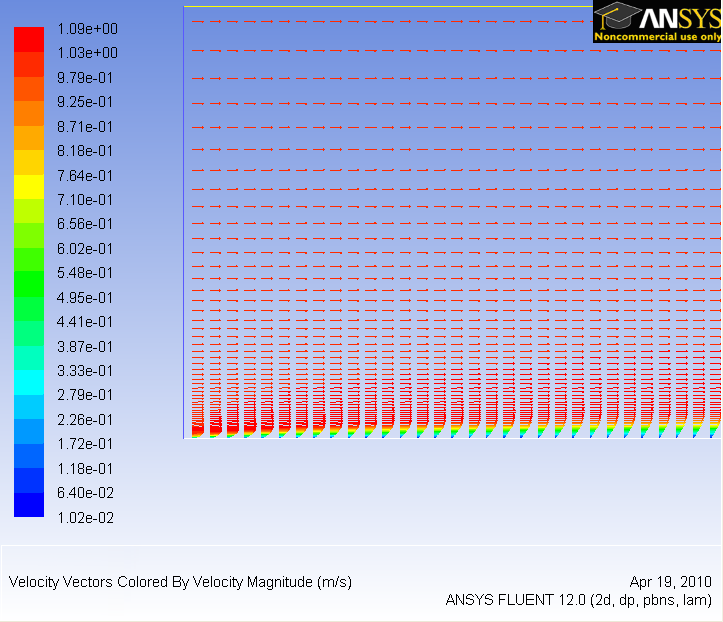Image Removed !step6_1.png|width=298,height=257!Higher Resolution Image

Remember to save the image using

...

Select Pressure...under Contours Of. Then select Pressure Coefficient from the second drop-down menu. Also, check the Filled checkbox and set Levels to 90. Then click on Display to update the display window.
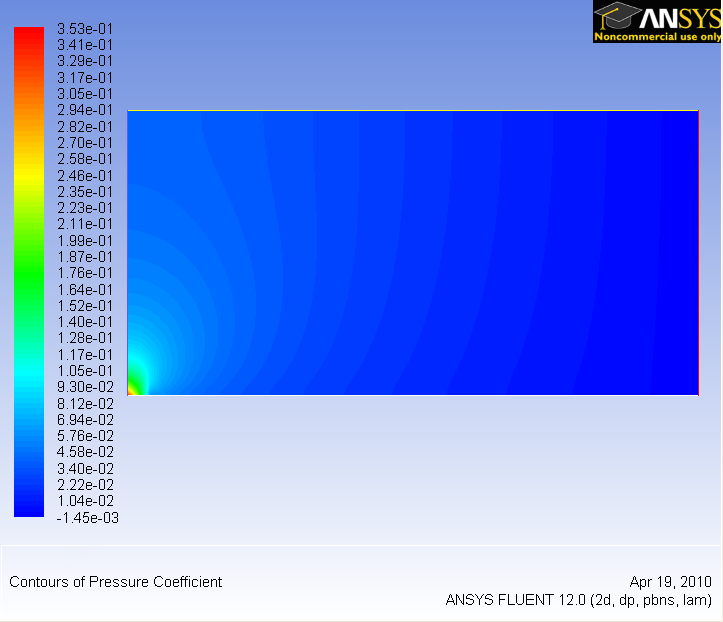Image Removed !step6_002.png|width=295,height=255!Higher Resolution Image

Zoom in at the leading edge. 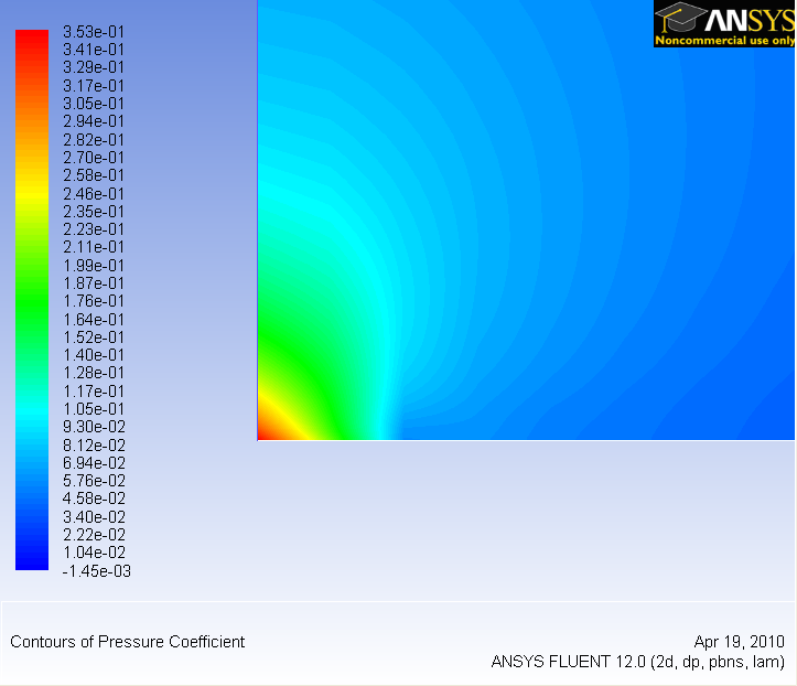Image Removed. !step6_003.png|width=297,height=256!Higher Resolution Image

Why is the pressure not constant at the leading edge of the plate?

...

Now, compare your solution to the with the Blasius solution's skin friction by loading the file and then plotting it with your solution. (Download file here)

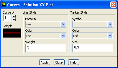
Also, you can change the symbol into lines by going to Curves... and click on the corresponding pattern that you like. Increase the Weight to 3 for readability. Both results should be fairly similar. 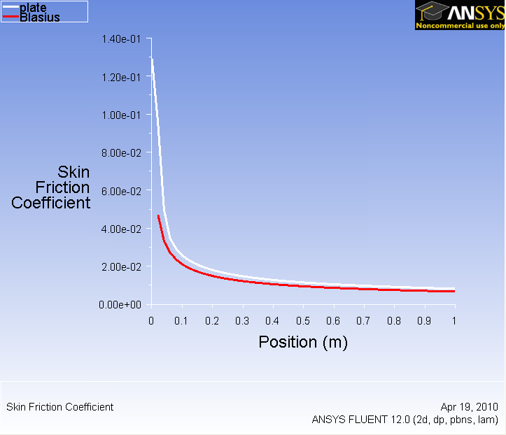Image Removed!step6_007.png|width=296,height=254!Higher Resolution Image

Now we will look at the velocity along the plate at outlet.

...

Uncheck Position on X Axis and check Position on Y Axis under Options. Under Plot Direction, set X to 0 and Y to 1. Under X Axis Function, select Velocity...Then, change Velocity Magnitude to X Velocity. Finally under surface, select outlet. Before we are ready to plot, click on the Axes... button and rescale the y-axis from 0 to 0.12. Also, check the Major Rules and Minor Rules for both axes. Remember that you must click the Apply button when performing changes in each axis.

Click Plot. 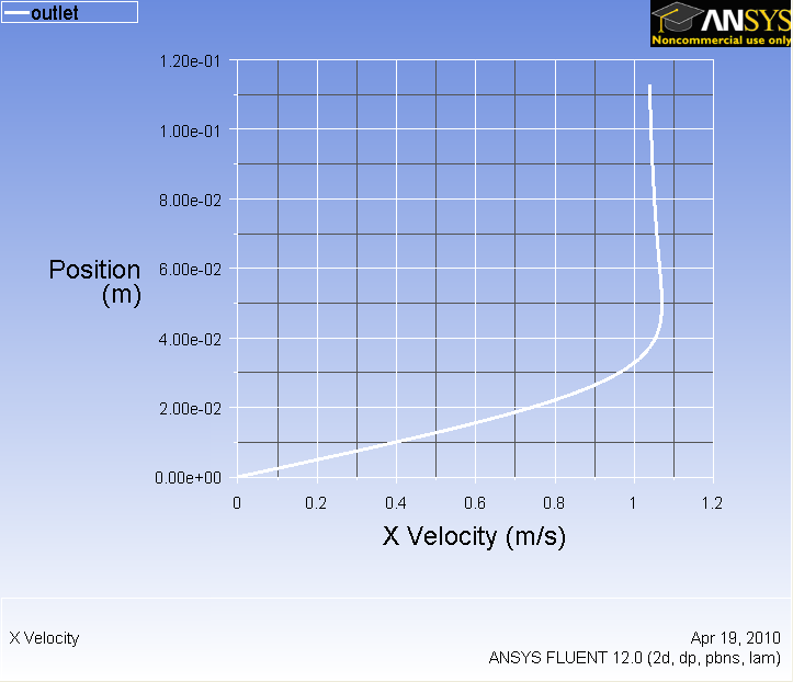Image Removed. !step6_008.png|width=297,height=255!Higher Image Resolution

To compare with the Blasius solution, download the solution here. Click Load File...and select the file you just downloaded. Then plot the solutions again to display both lines on the same graph. 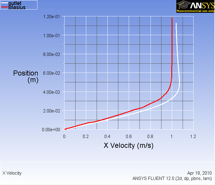Image Removed. !step6_009.png|width=298,height=256!Higher Resolution Image

What is the noticeably different between two solutions? Why is the velocity overshoot 1 for FLUENT's solution?

...

Under Surfaces, select outlet and {}x_0.5 and Plot. 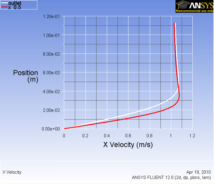Image Removed. !step6_010.png|width=299,height=257!Higher Resolution Image

Go to Step 7: Verify Results