 Sign-up for free online course on ANSYS simulations!
| Include Page |
|---|
...
|
...
|
| Panel |
|---|
Author: John Singleton and Rajesh Bhaskaran, Cornell University Problem Specification |
| Info | ||
|---|---|---|
| ||
We will use CFD-Post as the primary post processing GUI. Steps for post processing in FLUENT can be found here. |
Step 6. Results
Double click on Results from the Workbench Window to launch CFD-Post.
Velocity Vectors
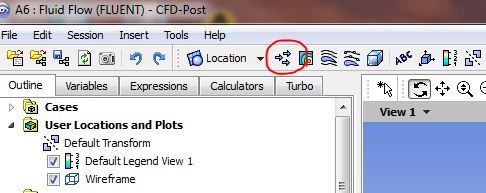
Click on the z-axis,  to view the XY plane. Click on the vector icon to insert a vector plot. Name it Velocity Vector.
A panel named "Details of Velocity Vector" will appear right below the outline window. Set the Locations to symmetry 1. Click on Apply to display the velocity vectors.
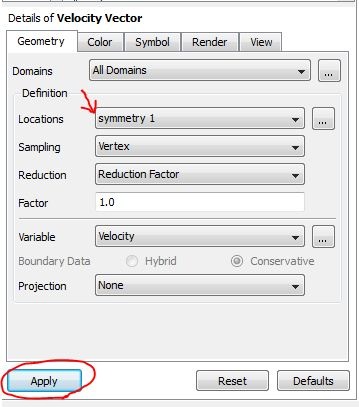
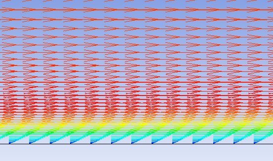
The velocity vectors will be displayed in the view window.

You can use the wheel button of the mouse to zoom into the region that closely surrounds the plate, to get a better view of the boundary layer velocities:
Outlet Velocity Profile
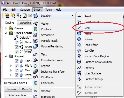
From the menu, insert > location > line. Name it "Outlet"
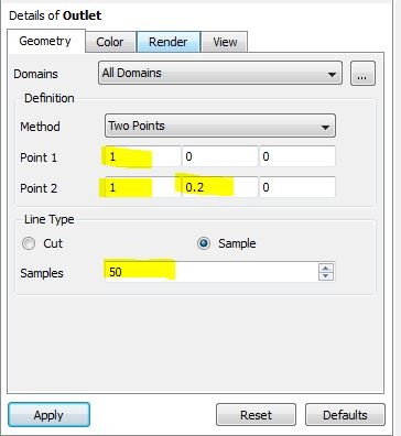
In the Details of Outlet panel, enter the following coordinates. Change the number of samples to 50. Click on Apply to create a line at the outlet.
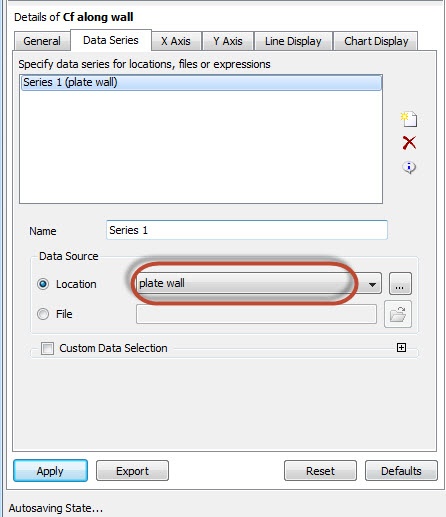
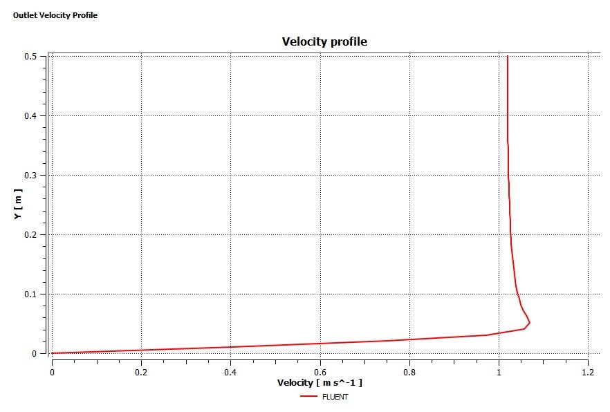
Insert a chart from the menu: insert > chart. Name the chart "Outlet Velocity Profile". Change the title to "Velocity Profile" in the General tab. In the Data Series tab, rename Series 1 to FLUENT and select Outlet for location. Select Velocity as the variable in the X Axis tab and select Y as the variable in the Y Axis tab. Click on Apply to generate the chart.
The velocity profile at the outlet is shown below:
We would like to compare the FLUENT result to the Blasius boundary layer solution. Download the Blasius solution here. Return to the Data Series tab and insert another data set. Rename it Blasius. Instead of specifying the location of the data, select the Blasius solution file you have downloaded.
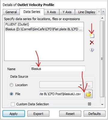
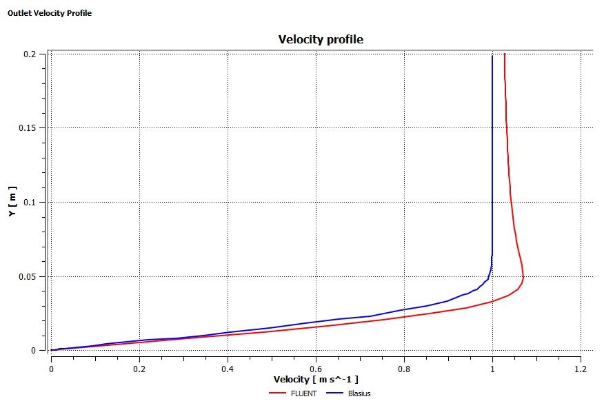
Click on Apply. The comparison should look like the following plot:
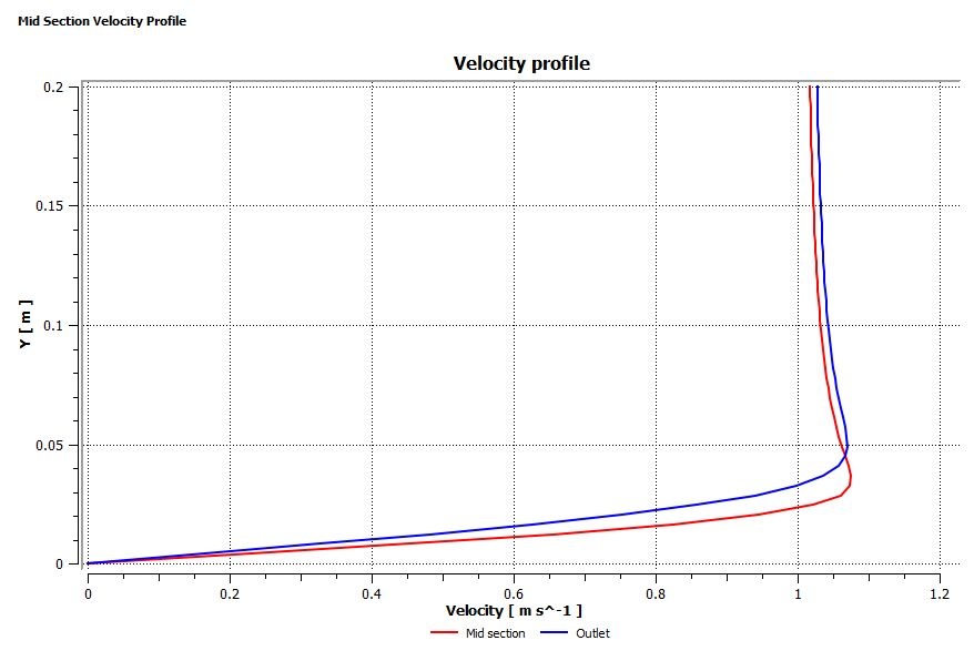
Mid-Section Velocity Profile
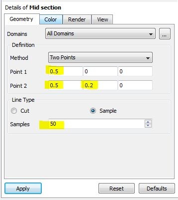
Here, we will plot the variation of the x component of the velocity along a vertical line in the middle of the geometry. In order to create the profile, we must first create a vertical line at x=0.5m. Insert another line, same as the previous step, and name it Mid section. Enter the following numbers to create a vertical line at x=0.5m. Set the number of samples to 50. Remember to click on Apply to finish.
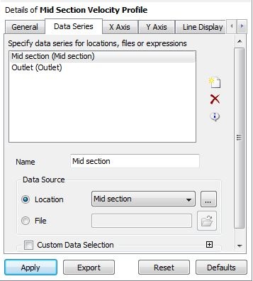
Insert another chart and name it Mid Section Velocity Profile. In the General tab, change the title to "Velocity profile". Select Mid Section as the location and rename Series 1 to Mid section. We will compare the velocity profiles at the mid section and at the outlet. Repeat the procedure in the previous step to insert the velocity profile at the outlet. Change the variable to Velocity in the X Axis tab and change the variable to Y in the Y Axis tab. Click on Apply to generate the chart.
The velocity profile comparison is shown below:
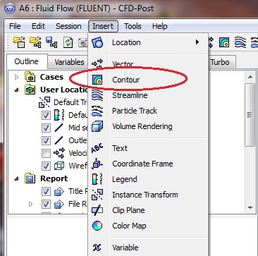
Pressure Contour
Insert > Contour. Name it Pressure contour.
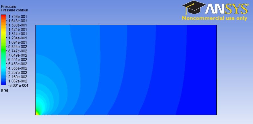
In Details of Pressure contour, change the locations to symmetry 1, change the variable to Pressure, and change the number of contours to 50.
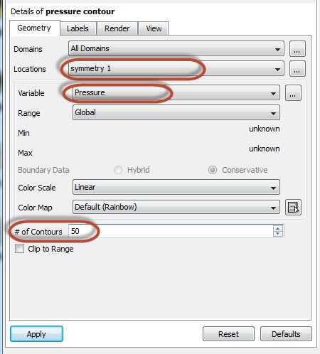
Click on Apply to view the contour.
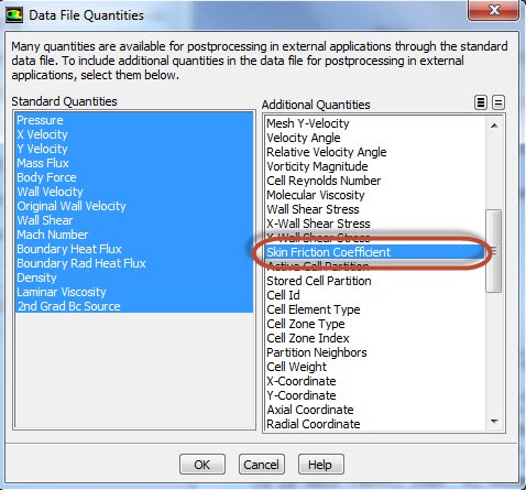
Skin Friction Coefficient
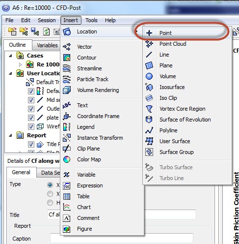
In FLUENT post processor the skin friction coefficient can be plotted as a function of distance along the plate. In CFD post, we can find the skin friction coefficient at each point along the axis. To create a point, click on Insert > Location > Point. Name it wall point.
In details of Point, retain the default XYZ value, (0,0,0), and click on Apply.
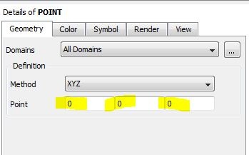
A point will be created at the coordinate (0,0,0), which is at the lower left corner of the solution domain.
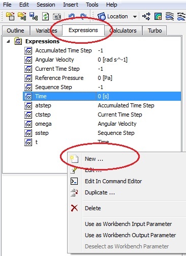
In the expression tab, create a new expression by right click in the expression window and select "new". Name it Wall shear.
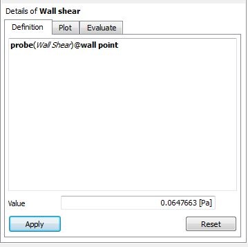
In Details of Wall shear, right below the Expressions window, enter the following and click on Apply. The value for the wall shear stress will be displayed.
We will now define the dynamic pressure. Create another expression and name it Dynamic pressure. In Details of Dynamic pressure, enter the following and click on Apply.
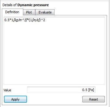
It is important to enter the appropriate units so the dynamic pressure has the correct unit. Recall both the density and the upstream velocity are set to 1.
The skin friction coefficient is the wall shear stress divided by the dynamic pressure. Create another expression and name it Cf. Enter the following and click on Apply.
| Include Page | ||||
|---|---|---|---|---|
|
Post Processing
Plot Velocity Vectors and Contours
| HTML |
|---|
<iframe width="560" height="315" src="https://www.youtube.com/embed/DCbh6z1v1wY" frameborder="0" allow="accelerometer; autoplay; encrypted-media; gyroscope; picture-in-picture" allowfullscreen></iframe> |
Note: In the below video (Plot Pressure Contours), please note that the cursor disappears accidentally at the 44 second mark and returns at the 3 minute mark. At 1 minute 17 seconds, "here" refers to the bottom-middle of the region near the plate. It is later drawn at the 1 minute 28 second mark. At 2 minute 40 seconds, "here" refers to the left most face, known as the inlet face, of the region.
Plot Pressure Contours
| HTML |
|---|
<iframe width="560" height="315" src="https://www.youtube.com/embed/KRQ0rtKCJ3w" frameborder="0" allow="accelerometer; autoplay; encrypted-media; gyroscope; picture-in-picture" allowfullscreen></iframe> |
Plot Velocity Profiles
| HTML |
|---|
<iframe width="560" height="315" src="https://www.youtube.com/embed/t3p52LPLw-A" frameborder="0" allow="accelerometer; autoplay; encrypted-media; gyroscope; picture-in-picture" allowfullscreen></iframe> |
Explanation for Velocity Profile Overshoot
| HTML |
|---|
<iframe width="560" height="315" src="https://www.youtube.com/embed/LnIsw07iuew?rel=0" frameborder="0" allowfullscreen></iframe> |
Check Similarity Principle
| HTML |
|---|
<iframe width="560" height="315" src="https://www.youtube.com/embed/Qde3pryaQ2A" frameborder="0" allow="accelerometer; autoplay; encrypted-media; gyroscope; picture-in-picture" allowfullscreen></iframe> |
Plot Velocity Derivatives
| HTML |
|---|
<iframe width="560" height="315" src="https://www.youtube.com/embed/kn6zk0AWsps" frameborder="0" allow="accelerometer; autoplay; encrypted-media; gyroscope; picture-in-picture" allowfullscreen></iframe> |
Calculate Drag Coefficient
| HTML |
|---|
<iframe width="560" height="315" src="https://www.youtube.com/embed/YrMyfB6n_W0" frameborder="0" allow="accelerometer; autoplay; encrypted-media; gyroscope; picture-in-picture" allowfullscreen></iframe> |
The skin friction coefficient is a dimensionless parameter. The value is 0.129533 at the point (0,0,0).
Go to Step 7: Verification & ValidationSee and rate the complete Learning Module