 Sign-up for free online course on ANSYS simulations!
...
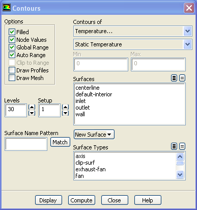
Select Pressure... and Static Pressure under Contours of. Use Levels of 30
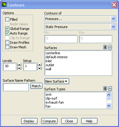
Click Display.

Notice that the pressure decreases as it flows to the right.
...
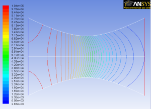
Select Pressure... and Total Pressure under Contours of. Select Filled. Use Levels of 100.
Click Display.

Around the nozzle outlet, we see that there is a pressure loss because of the numerical dissipation.
...
Select Temperature... and Static Temperature under Contours of. Use Levels of 30.
Click Display.
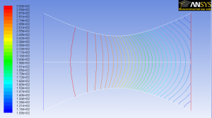

As we can see, the temperature decreases from left to right in the nozzle, indicating a transfer of internal energy to kinetic energy as the fluid speeds up.
...
Select Temperature.. .and Total Temperature under Contours of. Select Filled. Use Levels of 100.
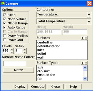
Click Display.

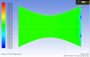
Looking at the scale, we see that the total temperature is uniform 300 K throughout the nozzle. The contour abnormality at the outlet of the nozzle is due to the round off errors.
...
Select Velocity...under Contours of and select Mach Number. Set Levels to 30.
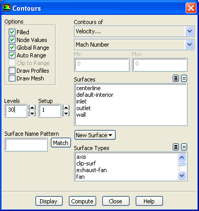
Click Display.
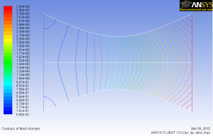

For 1D case, mach number is a function of x position. For 1D case, we are supposed to see vertical contour of mach numbers that are parallel to each other.
...
On the XY Plot window click on the Curves button. Change the Pattern to a line, Select a blank as a Symbol and change the Weight to any number greater than 2. To do this for multiple curves use the arrow buttons to navigate through the different curves displayed on the plot.

It is good to write the data into a file to have greater flexibility on how to present the result in the report. At the same XY Plot windows, select Write to File. Then click Write... Name the file "p.xy" in the directory that you prefer.
Open "p.xy" file with notepad or other word processing software. At the top, we see:
...
| Note | ||
|---|---|---|
| ||
The green line in the plot below SHOULD be in symbols. This will be corrected soon. |

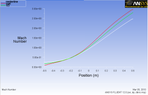
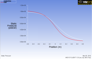
How does the FLUENT solution compare with the 1D solution?
...