Page History

...

...

For each mesh, take note of the drag coefficient and compare with each other.

We clearly see a difference in the drag coefficients, as the "Fine" case moves closer to the Experimental Data.

...

Let's analyze pressure coefficient plot around the spheres again. Use the same steps as before however, we want to overlay the corresponding result from the coarser mesh so that we can compare them. To do this, after plottting plotting the fine mesh results, in the Solution XY Plot, click on Load File. Navigate to your working folder, and click on the appropriate filename for the previous resulting coarse mesh, eg. press_coeff.xy and click OK. Also make sure we load the experimental data as well.

Click Plot. (If you cannot run the longer mesh, HERE is the XY file for the fine mesh so you can load it into the coarser mesh case and see the results next to each other).

Image Added

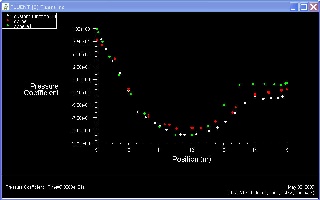
Note:  The green data ("Sphere1") is the experimental, the red ("Cpline") is the course case, and the white is the fine case data. Image Removed

We see that the Pressure Coefficient doesn't change all that much, so the correlation between mesh density and Pressure Coefficient accuracy is not that strong (but only for this case). The key difference lies in the change in the Drag coefficients we found earlier.

...