 Sign-up for free online course on ANSYS simulations!
...
| Panel |
|---|
Author: Daniel Kantor and Andrew Einstein, Cornell University Problem Specification |
...
We'll re-do the calculation on a 570,000 element mesh. IMPORTANT NOTE: Running a mesh this size with our element type will take at least week to run on a single PC. You can try running smaller size meshes on your own but the results will not be as good as these. You can download the mesh HERE. If you want to create it, follow Step 1 through Step 53. At step 2, you can simply change the cell size from 0.8 to 0.4 .
After that, you should have three meshes with following mesh elements.
...
Coarse
...
Medium
...
Fine
...
No. of cells
...
6240
...
14040
...
31590
IMPORTANT NOTE: Repeat steps 4, and 5 except there is a change in the ITERATE step. The Time Step Size will be changed to 0.01, the Number of Time Steps will be changed to 10,000, and the Max Iterations per Time Step will be changed to 15. Click Iterate and come back in a week (at least).
Repeat step 6 of the tutorial and plot each of the graphs as before.
Drag Coefficient Comparison
For each mesh, take note of the drag coefficient and compare with each other.
Experimental | 0.1 | ||
Coarse | Coarse | Medium | Fine |
Cd | 2.4981 | 2.4941 | 2.4927 |
% dif | 0.160378 4485 0 | ||
Fine | 0.056132 3733 |
We clearly see a difference in the drag coefficients, as the "Fine" case moves closer to the Experimental DataTaking medium as benchmark, we compare coarse and fine mesh. Note that the difference in drag coefficient between three meshes is negligibly small. For analysis of drag coefficient, it seems that coarse mesh provides enough resolution.
Pressure Coefficient Comparison
Let's analyze pressure coefficient plot around cylinder for three different mesh before we conclude which mesh to use. Let's start with a coarse mesh.
Plot > XY Plot...
Change the Y Axis Function to Pressure..., followed by Pressure Coefficient. Then, select cylinder under Surfaces. Check the option Write to File.
Click Write...
Enter the file name and directory to save.
Do the same for medium and fine meshes by opening different case and data files.
After that, open the files that you have written with excel spreadsheet. Compile and plot the data accordingly.
...
A quick and dirty way plotting three different mesh is to use FLUENT directly. Plot > XY Plot... You can Load File... that you have saved previously. However, using this way, you have less control of how you can present the data and is not recommended for report presentation.
the spheres again. Use the same steps as before however, we want to overlay the corresponding result from the coarser mesh so that we can compare them. To do this, after plotting the fine mesh results, in the Solution XY Plot, click on Load File. Navigate to your working folder, and click on the appropriate filename for the previous resulting coarse mesh, eg. press_coeff.xy and click OK. Also make sure we load the experimental data as well.
Click Plot. (If you cannot run the longer mesh, HERE is the XY file for the fine mesh so you can load it into the coarser mesh case and see the results next to each other).
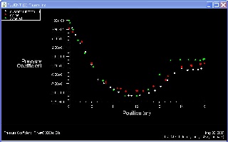
Note: The green data ("Sphere1") is the experimental, the red ("Cpline") is the course case, and the white is the fine case data.
We see that the Pressure Coefficient doesn't change all that much, so the correlation between mesh density and Pressure Coefficient accuracy is not that strong (but only for this case). The key difference lies in the change in the Drag coefficients we found earlier.