 Sign-up for free online course on ANSYS simulations!
...
UNDER
...
CONSTRUCTION
| Panel |
|---|
| }
Author: Daniel Kantor and Andrew Einstein, Cornell University Problem Specification |
Step 6: Analyze Results
For all of our analysis we will be looking at the Sphere surface under Surfaces, unless otherwise noted.
Plot Velocity Vectors
Let's plot the velocity vectors obtained from the FLUENT solution.
Display > Vectors
Set the Scale to 1 and Skip to 0. Click Display.
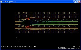
If we look closely at the sphere we can start to see where the separation occurs.
| Info | ||
|---|---|---|
| ||
Now, let's take a look at the Contour of Velocity magnitude around the sphere.
Display > Contours
Under Contours of, choose Velocity... and Velocity Magnitude. Select the Filled option. Increase the number of contour levels plotted: set Levels to 100.
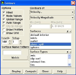
Click Display.
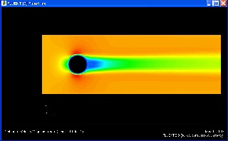
We see the flow is mostly what we would expect in this case.
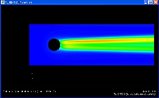
Now, let's take a look at the Contour of Turbulent Intensity around the sphere. This will give us a picture of the turbulence that is occurring around the sphere.
Display > Contours
Under Contours of, choose Turbulence... and Turbulent Intensity. Select the Filled option. Increase the number of contour levels plotted: set Levels to 100.
Click Display.
Pressure Coefficient
Pressure coefficient is a dimensionless parameter defined by the equation where p is the static pressure, p ref is the reference pressure, and q ref is the reference dynamic pressure defined by
| Latex |
|---|
University {color:#ff0000}{*}Problem Specification{*}{color} [1. Create Geometry in GAMBIT|FLUENT - Turbulent Flow Past a Sphere - Step 1] [2. Mesh Geometry in GAMBIT|FLUENT - Turbulent Flow Past a Sphere - Step 2] [3. Specify Boundary Types in GAMBIT|FLUENT - Turbulent Flow Past a Sphere - Step 3] [4. Set Up Problem in FLUENT|FLUENT - Turbulent Flow Past a Sphere - Step 4] [5. Solve\!|FLUENT - Turbulent Flow Past a Sphere - Step 5] [6. Analyze Results|FLUENT - Turbulent Flow Past a Sphere - Step 6] [7. Refine Mesh|FLUENT - Turbulent Flow Past a Sphere - Step 7] [Problem 1|FLUENT - Turbulent Flow Past a Sphere - Problem 1] {panel} h2. Step 6: Analyze Results For all of our analysis we will be looking at the {color:#660099}{*}{_}Sphere{_}{*}{color} surface under {color:#660099}{*}{_}Surfaces{_}{*}{color}, unless otherwise noted. h4. Plot Velocity Vectors Let's plot the velocity vectors obtained from the FLUENT solution. *Display > Vectors* Set the {color:#660099}{*}{_}Scale{_}{*}{color} to 1 and {color:#660099}{*}{_}Skip{_}{*}{color} to 0. Click {color:#660099}{*}{_}Display{_}{*}{color}. !Vectors.jpg|thumbnail! *If we look closely at the sphere we can start to see where the separation occurs.* {info:title=Zoom in the cylinder using the middle mouse button.} {info} Now, let's take a look at the Contour of Velocity magnitude around the sphere. *Display > Contours* Under {color:#660099}{*}{_}Contours of{_}{*}{color}, choose {color:#660099}{*}{_}Velocity..._{*}{color} and {color:#660099}{*}{_}Velocity Magnitude{_}{*}{color}. Select the {color:#660099}{*}{_}Filled{_}{*}{color} option. Increase the number of contour levels plotted: set {color:#660099}{*}{_}Levels{_}{*}{color} to {{100}}. !Contours.jpg|thumbnail! Click {color:#660099}{*}{_}Display{_}{*}{color}. \\ !VelocityMag.jpg|thumbnail! *We see the flow is mostly what we would expect in this case.* Now, let's take a look at the Contour of Turbulent Intensity around the sphere. This will give us a picture of the turbulence that is occurring around the sphere. \\ *Display > Contours* Under {color:#660099}{*}{_}Contours of{_}{*}{color}, choose {color:#660099}{*}{_}Turbulence..._{*}{color} and {color:#660099}{*}{_}Turbulent Intensity{_}{*}{color}. Select the {color:#660099}{*}{_}Filled{_}{*}{color} option. Increase the number of contour levels plotted: set {color:#660099}{*}{_}Levels{_}{*}{color} to {{100}}. Click {color:#660099}{*}{_}Display{_}{*}{color}. \\ !TurbulentInt.jpg|thumbnail!\\ \\ h4. h4. Pressure Coefficient Pressure coefficient is a dimensionless parameter defined by the equation !step6_cp_equation.gif|width=32,height=32! where _p_ is the static pressure, _p_ ~ref~ is the reference pressure, and _q_ ~ref~ is the reference dynamic pressure defined by {latex}\large $$ q_{ref} = {1 \over 2}{\rho_{ref}v_{ref}^2}$${latex} |
The
...
reference
...
pressure,
...
density,
...
and
...
velocity
...
are
...
defined
...
in
...
the
...
Reference
...
Values
...
panel
...
in
...
Step
...
5.
...
Let's
...
plot
...
pressure
...
coefficient
...
vs
...
x-direction
...
along
...
the
...
cylinder.
...
Plot
...
>
...
XY
...
Plot...
...
Change
...
the
...
Y
...
Axis
...
Function
...
to
...
Pressure
...
...
...
,
...
followed
...
by
...
Pressure
...
Coefficient
...
.
...
Then,
...
select Sphere under Surfaces.
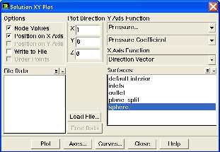
Click Plot.
We see that there is a lot of scatter in our data, so we will be creating a line along the sphere to try and get a better picture of the pressure coefficient. To accomplish this we will create a surface of Z-axis position zero, and plot the line y^2+(x-12)^2
...
-9,
...
which
...
is
...
the
...
equation
...
of
...
a
...
ring
...
around
...
the
...
sphere
...
in
...
the
...
x-y
...
plane.
...
Surface > Iso-Surface
...
Under Surface of Constant choose Grid...
...
and
...
Z-Coordinate
...
.
...
Under
...
Iso-Values
...
input
...
0
...
.
...
This
...
will
...
create
...
a
...
plane
...
in
...
our
...
flow
...
in
...
which
...
the
...
Z
...
coordinate
...
is
...
zero
...
everywhere.
...
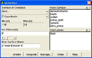
Call this Zero_Plane
...
and
...
click
...
Create
...
.
Define > Custom Field Functions
Here we input our formula y^2+(x-12)^2
...
-
...
9
...
under
...
Definition
...
.
...
To
...
do
...
use
...
the
...
Field
...
Functions
...
section
...
and
...
choose
...
Grid...
...
and
...
choose
...
X-Coordinate
...
and
...
Y-Coordinate
...
for
...
the
...
"x"
...
and
...
"y"
...
in
...
the
...
above
...
formula.
...
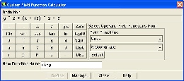
Call this Ring and click Define.
Surface > Iso-Surface
Now under Surface of Constant choose Custom Field Functions and choose our function Ring. Keep the default Iso-Values to 0. Then, within From Surfaces select Zero_Plane.
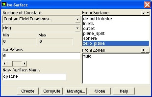
Call this CpLine and click Create.
We have now created the necessary line around the sphere to view the data better. Follow the same steps as before to plot the Pressure Coefficient, except that under Surfaces choose CpLine.
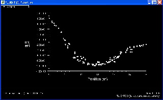
We now see that the data is has less scatter (this effect, however, is far more significant on a more refined mesh).

Comparison
With our simulation data, we can now compare the Fluent with experimental data. Click HERE to download the experimental data. The two sets of data for Pressure Coefficients are shown here:
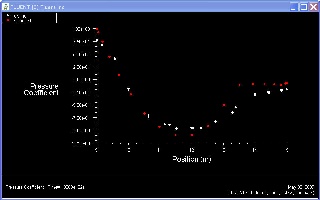
The Red dots are the experimental data (labeled "sphere1"), while the white dots are our data (labeled CPline).
Lets display the coefficient of drag:
Report > Forces
Make sure that under Force Vector the X has a 1 by it (this represents the drag on the sphere), and that under Wall Zones, sphere is highlighted.
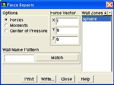
Click Print.
The two sets of data for drag coefficient are shown here:
Experimental | 0.1 |
Simulation | 0.4485 |