Page History

Step 6: Analyze Results

...

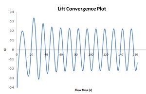
Lift convergence plot can be used to compute the correct value of Strouhal number. Non-dimensionalize the problem and Sr = f*D/U = 0.0846 0859 * 2 = 0.169172. The results matches fairly well with the value 0.183 as reported by Williamson

}
\large
$$
{\rm{Period}} = {{T_2 - T_1} \over {10}}
$$
{latex}\\

{latex}

\large
$$
{\rm{f}} = {{1} \over {Period}}$$

{latex}\\

{latex}
\large
$$
{\rm{Sr}} = {fD \over U}
$$
{latex}\\

An example of Lift Convergence Plot plotted using excel is shown below:

!Excel

 Lift convergence_sm.jpg!
 
{newwindow:Higher Resolution Image}https://confluence.cornell.edu/download/attachments/107011456107011458/Excel%20Lift%20convergence.jpg{newwindow}

Display Pressure Contours

Main Menu > Display > Contours
Image Removed Image Added

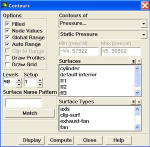
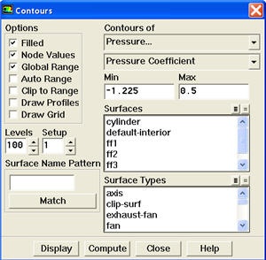
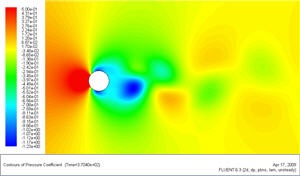
Under Contours of, choose Pressure.. and Static Pressure Coefficient. Select the Filled option. Increase the number of contour levels plotted: set Levels to 40. Set Levels to 100. Disable Auto Range and Clip to Range from the Options group box. Enter -1.225 and 0.5 for Min and Max, respectively.Click Display.
Image Removed

Image Added

https://confluence.cornell.edu/download/attachments/107011458/pressure%20contour%20plotpressure%20coefficient%20contour%20plot.jpg

The contour shows a clear asymmetric pattern in the flow.  The local pressure minima (the green patch downstream) are the center of the vortices.
 

Display Contour of Vorticity Magnitude

Main Menu > Display > Contours

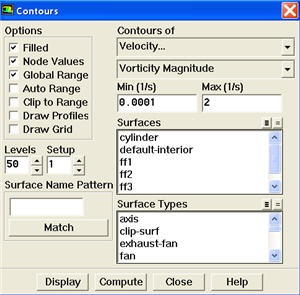
Under Contours of, choose Velocity.. and Vorticity Magnitude. Disable Auto Range and Clip to Range from the Options group box. Enter 0.0001 and 2 for Min and Max, respectively. Select Levels to 50. Click Display.

Image Added Image Removed

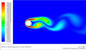
https://confluence.cornell.edu/download/attachments/107011458/velocity%20magnitude%20contour%20plotvorticity%20magnitude%20contour%20plot.jpg

This figure shows clear vortex shedding process. Zoom in the view around cylinder. 

...