 Sign-up for free online course on ANSYS simulations!
| Panel |
|---|
Problem Specification |
Step 5: Solve!
Set Solution Controls
Main Menu > Solve > Controls > Solution...
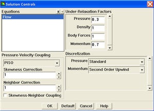
Select PISO from the Pressure-Velocity Coupling drop-down list.
| Info | ||
|---|---|---|
| ||
PISO allows the use of higher time step size without affecting the stability of the solution. Hence it is recommended pressure-velocity coupling for solving transient applications. |
Uncheck Skewnes-Neighbor Coupling.
Select Second Order Upwind from the Momentum drop-down list in the Discretization group box. Click OK to close the Solution Controls panel.
Set Initial Guess
Initialize the flow field to the values at the inlet:
Main Menu > Solve > Initialize > Initialize...
In the Solution Initialization menu that comes up, choose farfield1 under Compute From. The X Velocity for all cells will be set to 1 m/s, the Y Velocity to 0 m/s and the Gauge Pressure to 0 Pa. These values have been taken from the farfield1 boundary condition.
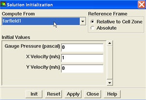
Click Init. This completes the initialization. Close the window.
Patch Region
We will patch the upper region downstream of the flow to create asymmetry so that we can obtain stable oscillation of vortex shedding faster.
To do this, we will create a register to patch the Y velocity in downstream of cylinder.
Main Menu > Adapt > Region...
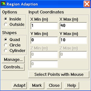
Enter 1 and 40 for X Min and X Max. Enter 0 and 10 for Y Min and Y Max. Click Mark. FLUENT will print the following message in the console window:
5416 cells marked for refinement, 0 cells marked for coarsening
Close the Region Adaption panel.
We will now patch Y velocity in the registered region.
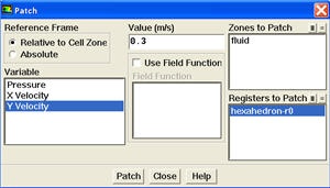
Main Menu > Solve > Initializate > Patch...
| newwindow | ||||
|---|---|---|---|---|
| ||||
| Wiki Markup | ||||
{panel} Author: Rajesh Bhaskaran & Yong Sheng Khoo, Cornell University [Problem Specification|FLUENT - Unsteady Flow Past a Cylinder - Problem Specification]\\ [1. Create Geometry in GAMBIT|Fluent - Unsteady Flow Past a Cylinder - Step 1]\\ [2. Mesh Geometry in GAMBIT|FLUENT - Unsteady Flow Past a Cylinder - Step 2]\\ [3. Specify Boundary Types in GAMBIT|FLUENT - Unsteady Flow Past a Cylinder - Step 3]\\ [4. Set Up Problem in FLUENT|FLUENT - Unsteady Flow Past a Cylinder - Step 4]\\ {color:#ff0000}{*}5. Solve\!*{color} [6. Analyze Results|FLUENT - Unsteady Flow Past a Cylinder - Step 6]\\ [7. Refine Mesh|FLUENT - Unsteady Flow Past a Cylinder - Step 7]\\ {panel} {dynamictable:UniqueName\|title=Table Title} \|\|header1\|\|header2\|\|header3\|\| {dynamictable} h2. Step 5: Solve\! h4. Set Solution Controls *Main Menu > Solve > Controls > Solution...* !solution control.jpg! Select {color:#660099}{*}{_}PISO{_}{*}{color} from the {color:#660099}{*}{_}Pressure-Velocity Coupling{_}{*}{color} drop-down list. {info:title= }PISO allows the use of higher time step size without affecting the stability of the solution. Hence it is recommended pressure-velocity coupling for solving transient applications. {info} Uncheck {color:#660099}{*}{_}Skewnes-Neighbor Coupling{_}{*}{color}. Select {color:#660099}{*}{_}Second Order Upwind{_}{*}{color} from the Momentum drop-down list in the {color:#660099}{*}{_}Discretization{_}{*}{color} group box. Click {color:#660099}{*}{_}OK{_}{*}{color} to close the {color:#660099}{*}{_}Solution Controls{_}{*}{color} panel. \\ h4. Set Initial Guess Initialize the flow field to the values at the inlet: *Main Menu > Solve > Initialize > Initialize...* In the _Solution Initialization_ menu that comes up, choose {color:#660099}{*}{_}inlet{_}{*}{color} under {color:#660099}{*}{_}Compute From{_}{*}{color}. The {color:#660099}{*}{_}X Velocity{_}{*}{color} for _all_ cells will be set to 1 m/s, the {color:#660099}{*}{_}Y{_}{*}{color} {color:#660099}{*}{_}Velocity{_}{*}{color} to 0 m/s and the {color:#660099}{*}{_}Gauge Pressure{_}{*}{color} to 0 Pa. These values have been taken from the inlet boundary condition. !Initialize.jpg! Click {color:#660099}{*}{_}Init{_}{*}{color}. This completes the initialization. {color:#660099}{*}{_}Close{_}{*}{color} the window. \\ h4. Patch Region We will patch the upper region downstream of the flow to create asymmetry so that we can obtain stable oscillation of vortex shedding faster. To do this, we will create a register to patch the Y velocity in downstream of cylinder. *Main Menu > Adapt > Region...* \\ !Region Adaption.jpg! Enter {{1}} and {{40}} for {color:#660099}{*}{_}X Min{_}{*}{color} and {color:#660099}{*}{_}X Max{_}{*}{color}. Enter {{0}} and {{10}} for {color:#660099}{*}{_}Y Min{_}{*}{color} and {color:#660099}{*}{_}Y Max{_}{*}{color}. Click {color:#660099}{*}{_}Mark{_}{*}{color}. FLUENT will print the following message in the console window: {{{_}5416 cells marked for refinement, 0 cells marked for coarsening{_}}} {color:#660099}{*}{_}Close{_}{*}{color} the _Region Adaption_ panel. We will now patch Y velocity in the registered region. *Main Menu > Solve > Initializate > Patch...* \\ !patch_sm.jpg! {newwindow:Higher Resolution Image}https://confluence.cornell.edu/download/attachments/107011456/patch.jpg {newwindow} Select {color:#660099}{*}{_} |
Select hexahedron-r0
...
from
...
the
...
Registers
...
to
...
Patch
...
.
...
Select
...
Y
...
Velocity
...
from
...
the
...
Variable
...
selection
...
list.
...
Enter
...
0.3
...
for Value. Click Patch.
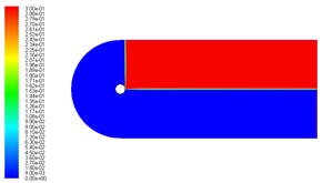
To check whether you have patch the region, plot contour of velocity in the y direction.
Main Menu > Display > Contours...
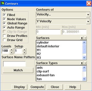
Select Velocity... and Y Velocity under Contours of drop-down list. Make sure to check the Filled under Options. Click Display.
| newwindow | ||||
|---|---|---|---|---|
| ||||
https://confluence.cornell.edu/download/attachments/107011456/display_patch.jpg |
As can be seen, the Y Velocity is zero everywhere except for the patched region, we have Y Velocity of 0.3 m/s.
Set Convergence Criteria
FLUENT reports a residual for each governing equation being solved. The residual is a measure of how well the current solution satisfies the discrete form of each governing equation. We'll iterate the solution until the residual for each equation falls below 1e-3.
Main Menu > Solve > Monitors > Residual...
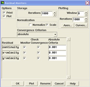
Default value for Convergence Criterion for continuity, x-velocity, and y-velocity is 1e-3.
Also, under Options, select Plot and Print. This will plot the residuals in the graphics window as they are calculated.
Click OK.
Monitor also the lift coefficient on the cylinder.
Main Menu > Solve > Monitors > Force...
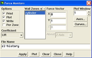
Under Coefficient, select Lift. Select cylinder under Wall Zones. Under Options, select Print, Plot and Write. Note that Plot Window is 1. Click Apply.
Set Reference Values
The reference values are used to non-dimensionalize the forces and moments action on the wall surface.
Main Menu > Reference Values...
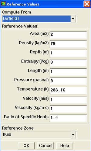
Select farfield1 from the Compute From drop-down list. FLUENT will update the reference values based on the boundary conditions at farfield1. Change Area to 2. Click OK.
| Info | ||
|---|---|---|
| ||
Note that cross sectional area for a 2D cylinder is the diameter of the cylinder. Setting the right area is important for getting correct drag coefficient. |
Set Animation Control (Optional)
Let's set the animation to observe the vorticity magnitude.
Main Menu > Solve > Animate > Define...
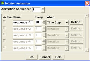
Increase the Animation Sequences to 1. Enter 10 for Every. Select Time Step from When drop-down list. Click Define... for sequence-1 to open the Animation Sequence panel.
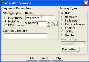
Increase Window to 2 and click the Set button to open a graphics window. Select Contours from the Display Type list to open the Contours panel. Select Velocity... and Vorticity Magnitude from the Contours of drop-down lists.
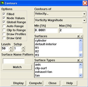
Disable Auto Range and Clip to Range from the Options group box. Enter 0.0001 and 2 for Min and Max, respectively. Select Levels to 50. Click Display. Click OK to close the Animation Sequence panel. Click OK to close the Solution Animation panel. This will save .hmf file after every 10 time steps. We can later create an animation in the form of movie clip using these files. Save the case and data files.
Main Menu > File > Write > Case & Data...
| Info | ||
|---|---|---|
| ||
We can review the animation created after we are done with iterations. Note that you don't necessarily get a good format when exporting to MPEG. It is advisable to use the available playback option. |
Iterate the Solution
Main Menu > Solve > Iterate...
You will have to input the time step size for iteration. Smaller time step means more accurate result but more computational time. We need to find the balance between accuracy and computational time.
| Info | ||||
|---|---|---|---|---|
| ||||
The Strouhal number for flow past cylinder is roughly 0.183 as reported by Williamson .
For our case, D = 2, U = 1
Therefore, Time Step Size = 10.9/25 = 0.436 sec ~ 0.4 sec |
Enter 0.4 for Time Step Size (s). Enter 30 for Max. Iterrations per Time Step. Enter 800 for Number of Time Steps. Click Apply. Click Iterate to start the iterations.
| newwindow | ||||
|---|---|---|---|---|
| ||||
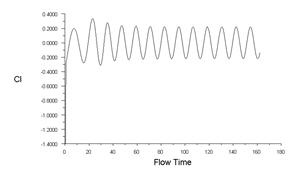
https://confluence.cornell.edu/download/attachments/107011456/Cl%20convergence.jpg |
We can see a clear sinusoidal pattern, a sign of sustained vortex shedding process after 40s. Stop the iteration after about 350s.
Save the case and solution.
Main Menu > File > Write > Case & Data...
Use the default name (Mesh's file name "cylinder") and click OK.