 Sign-up for free online course on ANSYS simulations!
| Panel |
|---|
Problem Specification |
Step 4: Set Up Problem in FLUENT
Launch Fluent
Lab Apps > FLUENT 6.3.26
Select 2ddp from the list of options and click Run.
| Panel |
|---|
The "2ddp" option is used to select the 2-dimensional, double-precision solver. In the double-precision solver, each floating point number is represented using 64 bits in contrast to the single-precision solver which uses 32 bits. The extra bits increase not only the precision but also the range of magnitudes that can be represented. The downside of using double precision is that it requires more memory. |
Import Grid
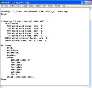
Main Menu > File > Read > Case...
Navigate to the working directory and select the cylinder.msh file. This is the mesh file that was created using the preprocessor GAMBIT in the previous step. FLUENT reports the mesh statistics as it reads in the mesh:
| newwindow | ||||
|---|---|---|---|---|
| ||||
| Wiki Markup | ||||
{panel} Author: Rajesh Bhaskaran & Yong Sheng Khoo, Cornell University [Problem Specification|FLUENT - Unsteady Flow Past a Cylinder - Problem Specification]\\ [1. Create Geometry in GAMBIT|Fluent - Unsteady Flow Past a Cylinder - Step 1]\\ [2. Mesh Geometry in GAMBIT|FLUENT - Unsteady Flow Past a Cylinder - Step 2]\\ [3. Specify Boundary Types in GAMBIT|FLUENT - Unsteady Flow Past a Cylinder - Step 3]\\ {color:#ff0000}{*}4. Set Up Problem in FLUENT{*}{color} [5. Solve\!|FLUENT - Unsteady Flow Past a Cylinder - Step 5]\\ [6. Analyze Results|FLUENT - Unsteady Flow Past a Cylinder - Step 6]\\ [7. Refine Mesh|FLUENT - Unsteady Flow Past a Cylinder - Step 7]\\ {panel}{slide:Fruit Is Good} \* Bananas are fruit \* Fruit is healthy \* Therefore, bananas are healthy {slide} {slide:title=More stuff\|hide=true} \* this slide still needs work {slide} h2. Step 4: Set Up Problem in FLUENT h4. Launch Fluent *Lab Apps > FLUENT 6.3.26* Select {color:#660099}{*}{_}2ddp{_}{*}{color} from the list of options and click {color:#660099}{*}{_}Run{_}{*}{color}. \\ {panel} The "2ddp" option is used to select the 2-dimensional, double-precision solver. In the double-precision solver, each floating point number is represented using 64 bits in contrast to the single-precision solver which uses 32 bits. The extra bits increase not only the precision but also the range of magnitudes that can be represented. The downside of using double precision is that it requires more memory. {panel} \\ h4. Import Grid *Main Menu > File > Read > Case...* Navigate to the working directory and select the cylinder.msh file. This is the mesh file that was created using the preprocessor _GAMBIT_ in the previous step. FLUENT reports the mesh statistics as it reads in the mesh: [!step4_img001sm.jpg!|^step4_img001.jpg]\\ {newwindow:Higher Resolution Image} https://confluence.cornell.edu/download/attachments/107011453/step4_img001.jpg{newwindow} |
Also,
...
take
...
a
...
look
...
under
...
zones.
...
We
...
can
...
see
...
the
...
five
...
zones
...
farfield1
...
,
...
farfield2
...
,
...
farfield3
...
,
...
farfield4
...
,
...
and
...
cylinder
...
that
...
we
...
defined
...
in
...
GAMBIT
...
.
...
Check
...
and
...
Display
...
Grid
...
First,
...
we
...
check
...
the
...
grid
...
to
...
make
...
sure
...
that
...
there
...
are
...
no
...
errors.
...
Main
...
Menu
...
>
...
Grid
...
>
...
Check
...
Any
...
errors
...
in
...
the
...
grid
...
would
...
be
...
reported
...
at
...
this
...
time.
...
Check
...
the
...
output
...
and
...
make
...
sure
...
that
...
there
...
are
...
no
...
errors
...
reported.
...
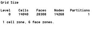
Check
...
the
...
grid
...
size:
...
Main
...
Menu
...
>
...
Grid
...
>
...
Info
...
>
...
Size
...
The
...
following
...
info
...
should
...
appear:
...
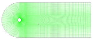
Display the grid:
Main Menu > Display > Grid...
...
Make
...
sure
...
all
...
6
...
items
...
under
...
Surfaces
...
is
...
selected.
...
Then
...
click
...
Display
...
.
...
The
...
graphics
...
window
...
opens
...
and
...
the
...
grid
...
is
...
displayed
...
in
...
it.
...
You
...
can
...
now
...
click
...
Close
...
in
...
the
...
Grid
...
Display
...
menu
...
to
...
get
...
back
...
some
...
desktop
...
space.
...
The
...
graphics
...
window
...
will
...
remain.
| Info | ||||||||
|---|---|---|---|---|---|---|---|---|
| =
|
|
| |||||
| }{*} Translation: *The grid can be translated in any direction by holding down the {color:#660099}{*}{_}Left Mouse Button {_}{*}{color}and then moving the mouse in the desired direction. *
In: *Hold down the {color:#660099}{*}{_}Middle Mouse Button {_}{*}{color}and drag a box from the {color:#660099}{*}{_}Upper Left Hand Corner {_}{*}{color}to the {color:#660099}{*}{_}Lower Right Hand Corner {_}{*}{color}over the area you want to zoom in on. *
Out: *Hold down the {color:#660099}{*}{_}Middle Mouse Button {_}{*}{color}and drag a box anywhere from the {color:#660099}{*}{_}Lower Right Hand Corner {_}{*}{color}to the {color:#660099}{*}{_}Upper Left Hand Corner. |
Use these operations to zoom into the grid to obtain the view shown below.
| Warning | ||
|---|---|---|
| ||
| newwindow | ||||
|---|---|---|---|---|
| ||||
{_}{*}{color}. {info} Use these operations to zoom into the grid to obtain the view shown below. {warning:title=The zooming operations can only be performed with a middle mouse button.} {warning} [!step4_img003sm.jpg!|^step4_img003.jpg] {newwindow:Higher Resolution Image} https://confluence.cornell.edu/download/attachments/107011453/step4_img003.jpg?version=1{newwindow} {tip:title=White Background on Graphics Window} To get white background go to: *Main Menu > File > Hardcopy* Make sure that {color:#660099}{*}{_}Reverse Foreground/Background{_}{*}{color} is checked and select {color:#660099}{*}{_}Color{_}{*}{color} in {color:#660099}{*}{_}Coloring{_}{*}{color} section. Click {color:#660099}{*}{_}Preview{_}{*}{color}. Click {color:#660099}{*}{_}No{_}{*}{color} when prompted "_Reset graphics window?_" {tip} You can also look at specific parts of the grid by choosing the boundaries you wish to view under {color:#660099}{*}{_}Surfaces{_}{*}{color} (click to select and click again to deselect a specific boundary). Click {color:#660099}{*}{_}Display{_}{*}{color} again when you have selected your boundaries. h4. Define Solver Properties *Main Menu > Define > Models > Solver* Under {color:#660099}{*}{_}Time{_}{*}{color}, select {color:#660099}{*}{_}Unsteady{_}{*}{color}. We will use the default {color:#660099}{*}{_}1st-Order Implicit{_}{*}{color}{color:#660099}{*}{_}Unsteady Formulation{_}{*}{color} for for now. Click {color:#660099}{*}{_}OK{_}{*}{color}. *Main Menu > Define > Models > Viscous* Laminar flow is the default. So we don't need to change anything in this menu. Click {color:#660099}{*}{_}Cancel{_}{*}{color}. *Main Menu > Define > Models > Energy* For incompressible flow, the energy equation is decoupled from the continuity and momentum equations. We need to solve the energy equation only if we are interested in determining the temperature distribution. We will not deal with temperature in this example. So leave the {color:#660099}{*}{_}Energy Equation{_}{*}{color} unselected and click {color:#660099}{*}{_}Cancel{_}{*}{color} to exit the menu. h4. Define Material Properties *Main Menu > Define > Materials...* Change {color:#660099}{*}{_}Density{_}{*}{color} to {{75}} and {color:#660099}{*}{_}Viscosity{_}{*}{color} to {{1}}. These are the values that we specified under [Problem Specification|FLUENT - Unsteady Flow Past a Cylinder - Problem Specification]. !material.jpg! Click {color:#660099}{*}{_}Change/Create{_}{*}{color}. Close the window. h4. Define Operating Conditions *Main Menu > Define > Operating Conditions...* For all flows, FLUENT uses gauge pressure internally. Any time an absolute pressure is needed, it is generated by adding the operating pressure to the gauge pressure. We'll use the default value of 1 atm (101,325 Pa) as the {color:#660099}{*}{_}Operating Pressure{_}{*}{color}. !step4_img005.jpg! Click {color:#660099}{*}{_}Cancel{_}{*}{color} to leave the default in place. h4. Define Boundary Conditions We'll now set the value of the velocity at the inlet and pressure at the outlet. Use the following table to set boundary type of each zone. | *Zone* | *Type* | | _farfield1_ | velocity-inlet, V ~x~ = 1 m/s | | _farfield2_ | velocity-inlet, V ~x~ = 1 m/s | | _farfield3_ | velocity-inlet, V ~x~ = 1 m/s | | _farfield4_ | pressure-outlet | | _cylinder_ | wall | *Main Menu > Define > Boundary Conditions...* Select {color:#660099}{*}{_}farfield1{_}{*}{color} under {color:#660099}{*}{_}Zone{_}{*}{color}. Change the {color:#660099}{*}{_}Type{_}{*}{color} of boundary as {color:#660099}{*}{_}velocity-inlet{_}{*}{color}. A new window will pop up. Change {color:#660099}{*}{_}Magnitude{_}{*}{color}, {color:#660099}{*}{_}Normal to Boundary to Components{_}{*}{color} under {color:#660099}{*}{_}Velocity Specification Method{_}{*}{color}. Input value _1_ next to {color:#660099}{*}{_}X-Velocity{_}{*}{color}. Click OK. Do the same for _farfield2_ and _farfield3_. \\ !step4_img006.jpg!\\ The (absolute) pressure at the farfield downstream is 1 atm. Since the operating pressure is set to 1 atm, the outlet gauge pressure = outlet absolute pressure - operating pressure = _0_. Choose {color:#660099}{*}{_}farfield4{_}{*}{color} under {color:#660099}{*}{_}Zone{_}{*}{color}. The {color:#660099}{*}{_}Type{_}{*}{color} of this boundary is {color:#660099}{*}{_}pressure-outlet{_}{*}{color}. Click on {color:#660099}{*}{_}Set..._{*}{color}. The default value of the {color:#660099}{*}{_}Gauge Pressure{_}{*}{color} is 0. Click {color:#660099}{*}{_}Cancel{_}{*}{color} to leave the default in place. Lastly, click on {color:#660099}{*}{_}cylinder{_}{*}{color} under {color:#660099}{*}{_}Zones{_}{*}{color} and make sure {color:#660099}{*}{_}Type{_}{*}{color} is set as {color:#660099}{*}{_}wall{_}{*}{color}. Click {color:#660099}{*}{_}Close{_}{*}{color} to close the _Boundary Conditions_ menu. *[*Go to Step 5: Solve\!*|FLUENT - Unsteady Flow Past a Cylinder - Step 5]* [See and rate the complete Learning Module|FLUENT - Unsteady Flow Past a Cylinder] [Go to all FLUENT Learning Modules|FLUENT Learning Modules] |
| Tip | ||
|---|---|---|
| ||
To get white background go to: |
You can also look at specific parts of the grid by choosing the boundaries you wish to view under Surfaces (click to select and click again to deselect a specific boundary). Click Display again when you have selected your boundaries.
Define Solver Properties
Main Menu > Define > Models > Solver
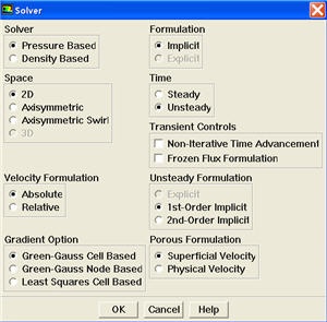
Under Time, select Unsteady. We will use the default 1st-Order ImplicitUnsteady Formulation for for now. Click OK.
Main Menu > Define > Models > Viscous
Laminar flow is the default. So we don't need to change anything in this menu. Click Cancel.
Main Menu > Define > Models > Energy
For incompressible flow, the energy equation is decoupled from the continuity and momentum equations. We need to solve the energy equation only if we are interested in determining the temperature distribution. We will not deal with temperature in this example. So leave the Energy Equation unselected and click Cancel to exit the menu.
Define Material Properties
Main Menu > Define > Materials...
Change Density to 75 and Viscosity to 1. These are the values that we specified under Problem Specification.
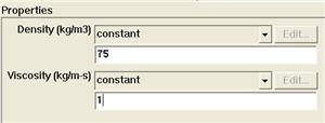
Click Change/Create. Close the window.
Define Operating Conditions
Main Menu > Define > Operating Conditions...
For all flows, FLUENT uses gauge pressure internally. Any time an absolute pressure is needed, it is generated by adding the operating pressure to the gauge pressure. We'll use the default value of 1 atm (101,325 Pa) as the Operating Pressure.
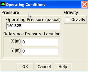
Click Cancel to leave the default in place.
Define Boundary Conditions
We'll now set the value of the velocity at the inlet and pressure at the outlet.
Use the following table to set boundary type of each zone.
Zone | Type |
farfield1 | velocity-inlet, V x = 1 m/s |
farfield2 | velocity-inlet, V x = 1 m/s |
farfield3 | velocity-inlet, V x = 1 m/s |
farfield4 | pressure-outlet |
cylinder | wall |
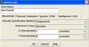
Main Menu > Define > Boundary Conditions...
Select farfield1 under Zone. Change the Type of boundary as velocity-inlet. A new window will pop up. Change Magnitude, Normal to Boundary to Components under Velocity Specification Method. Input value 1 next to X-Velocity. Click OK. Do the same for farfield2 and farfield3.
The (absolute) pressure at the farfield downstream is 1 atm. Since the operating pressure is set to 1 atm, the outlet gauge pressure = outlet absolute pressure - operating pressure = 0. Choose farfield4 under Zone. The Type of this boundary is pressure-outlet. Click on Set.... The default value of the Gauge Pressure is 0. Click Cancel to leave the default in place.
Lastly, click on cylinder under Zones and make sure Type is set as wall.
Click Close to close the Boundary Conditions menu.