 Sign-up for free online course on ANSYS simulations!
| Wiki Markup |
|---|
{alias:pipe1}
{panel}
|
| Panel |
Author: Rajesh Bhaskaran, CornellUniversity Problem Specification |
Problem Specification

Consider fluid flowing through a circular pipe of constant cross-section. The pipe diameter D=0.2 m and length L=8 m. The inlet velocity Vin=1 m/s. Consider the velocity to be constant over the inlet cross-section. The fluid exhausts into the ambient atmosphere which is at a pressure of 1 atm. Take density ρ=1 kg/ m3 and coefficient of viscosity µ= 2 x 10^-3^ kg/(ms). The Reynolds number Re based on the pipe diameter is
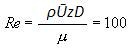
where V~avg~ is the average velocity at the inlet, which is 1m/s in this case.
Solve this problem using FLUENT. Plot the centerline velocity, wall skin-friction coefficient, and velocity profile at the outlet. Validate your results.
Note: The values used for the inlet velocity and flow properties are chosen for convenience rather than to reflect reality. The key parameter value to focus on is the Reynolds no.
Preliminary Analysis
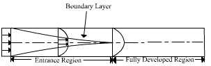
We expect the viscous boundary layer to grow along the pipe starting at the inlet. It will eventually grow to fill the pipe completely (provided that the pipe is long enough). When this happens, the flow becomes fully-developed and there is no variation of the velocity profile in the axial direction, x (see figure below). One can obtain a closed-form solution to the governing equations in the fully-developed region. You should have seen this in the Introduction to Fluid Mechanics course. We will compare the numerical results in the fully-developed region with the corresponding analytical results. So it's a good idea for you to go back to your textbook in the Intro course and review the fully-developed flow analysis. What are the values of centerline velocity and friction factor you expect in the fully-developed region based on the analytical solution? What is the solution for the velocity profile?
We'll create the geometry and mesh in GAMBIT which is the preprocessor for FLUENT, and then read the mesh into FLUENT and solve for the flow solution.
Go to Step 1: Create Geometry in GAMBIT
See and rate the complete Learning Module
...
 University

{color:#ff0000}{*}Problem Specification{*}{color}
[1. Create Geometry in GAMBIT|FLUENT - Laminar Pipe Flow Step 1]
[2. Mesh Geometry in GAMBIT|FLUENT - Laminar Pipe Flow Step 2]
[3. Specify Boundary Types in GAMBIT|FLUENT - Laminar Pipe Flow Step 3]
[4. Set Up Problem in FLUENT|FLUENT - Laminar Pipe Flow Step 4]
[5. Solve\!|FLUENT - Laminar Pipe Flow Step 5]
[6. Analyze Results|FLUENT - Laminar Pipe Flow Step 6]
[7. Refine Mesh|FLUENT - Laminar Pipe Flow Step 7]
[Problem 1|FLUENT - Laminar Pipe Flow Problem 1]
[Problem 2|FLUENT - Laminar Pipe Flow Problem 2]
{panel}

h2. Problem Specification

!Fluent_pipeflow.jpg!

Consider fluid flowing through a circular pipe of constant cross-section.         The pipe diameter _D_=0.2 m and length _L_=8 m. The inlet velocity _V{_}{_}{~}in{~}_=1         m/s. Consider the velocity to be constant over the inlet cross-section.         The fluid exhausts into the ambient atmosphere which is at a pressure         of 1 atm. Take density _ρ_=_1 kg/ m{_}{_}{^}3{^}_ and coefficient         of viscosity _µ= 2 x 10^-3\^ kg/(ms)._ The         Reynolds number _Re_ based on the pipe diameter is

!Fluent_Eq.jpg!

where _V~avg~_ is the average velocity at the inlet, which is 1m/s in this case.

Solve this problem using FLUENT. Plot the centerline velocity, wall         skin-friction coefficient, and velocity profile at the outlet. Validate         your results.

Note: The values used for the inlet velocity and flow properties are         chosen for convenience rather than to reflect reality. The key parameter         value to focus on is the Reynolds no.

h2. Preliminary Analysis

We expect the viscous boundary layer to grow along the pipe starting         at the inlet. It will eventually grow to fill the pipe completely (provided         that the pipe is long enough). When this happens, the flow becomes fully-developed         and there is no variation of the velocity profile in the axial direction, _x_ (see         figure below). One can obtain a closed-form solution to the governing         equations in the fully-developed region. You should have seen this in         the _Introduction to Fluid Mechanics_ course. We will compare the         numerical results in the fully-developed region with the corresponding         analytical results. So it's a good idea for you to go back to your textbook         in the Intro course and review the fully-developed flow analysis. What         are the values of centerline velocity and friction factor you expect         in the fully-developed region based on the analytical solution? What         is the solution for the velocity profile?

!TurbulentPipe.jpg!

We'll create the geometry and mesh in GAMBIT which is the preprocessor         for FLUENT, and then read the mesh into FLUENT and solve for the flow         solution.

Go to [Step 1: Create Geometry in GAMBIT|FLUENT - Laminar Pipe Flow Step 1]

[See and rate the complete Learning Module|FLUENT - Laminar Pipe Flow]

[Go to all FLUENT Learning Modules|FLUENT Learning Modules] |