 Sign-up for free online course on ANSYS simulations!
Step 5: Solve!
We'll use a second-order discretization scheme.
Main Menu > Solve > Controls > Solution...
Change Momentum to Second Order Upwind.
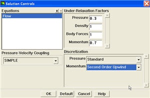
Click OK.
Set Initial Guess
Initialize the flow field to the values at the inlet:
Main Menu > Solve > Initialize > Initialize...
In the Solution Initialization menu that comes up, choose inlet under Compute From. The X Velocity for all cells will be set to 1 m/s, the Y Velocity to 0 m/s and the Gauge Pressure to 0 Pa. These values have been taken from the inlet boundary condition.
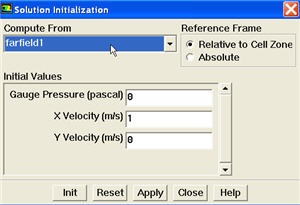
Click Init. This completes the initialization. Close the window.
Set Convergence Criteria
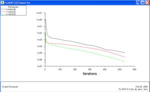
FLUENT reports a residual for each governing equation being solved. The residual is a measure of how well the current solution satisfies the discrete form of each governing equation. We'll iterate the solution until the residual for each equation falls below 1e-6.
Main Menu > Solve > Monitors > Residual...
Change the residual under Convergence Criterion for continuity, x-velocity, and y-velocity, all to 1e-5.
Also, under Options, select Plot. This will plot the residuals in the graphics window as they are calculated.
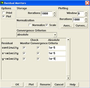
Click OK.
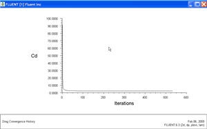
Monitor also the drag coefficient on the cylinder.
Main Menu > Solve > Monitors > Force...
Select cylinder under Wall Zones. Under Options, select Plot and Write. Note that Plot Window is 1.
Setting Reference Values
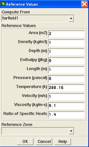
To plot C d, we need to set the reference value.
| Latex |
|---|
| Wiki Markup |
{panel} [Problem Specification|FLUENT - Steady Flow Past a Cylinder - Problem Specification]\\ [1. Create Geometry in GAMBIT|FLUENT - Steady Flow Past a Cylinder - Step 1]\\ [2. Mesh Geometry in GAMBIT|FLUENT - Steady Flow Past a Cylinder - Step 2]\\ [3. Specify Boundary Types in GAMBIT|FLUENT - Steady Flow Past a Cylinder - Step 3]\\ [4. Set Up Problem in FLUENT|FLUENT - Steady Flow Past a Cylinder - Step 4]\\ {color:#ff0000}{*}5. Solve\!*{color}\\ [6. Analyze Results|FLUENT - Steady Flow Past a Cylinder - Step 6]\\ [7. Refine Mesh|FLUENT - Steady Flow Past a Cylinder - Step 7]\\ [Problem 1|FLUENT - Steady Flow Past a Cylinder - Problem 1]\\ [Problem 2|FLUENT - Steady Flow Past a Cylinder - Problem 2] {panel} h2. Step 5: Solve\! We'll use a second-order discretization scheme. *Main Menu > Solve > Controls > Solution...* Change {color:#660099}{*}{_}Momentum{_}{*}{color} to {color:#660099}{*}{_}Second Order Upwind{_}{*}{color}. !step5_img001.jpg! Click {color:#660099}{*}{_}OK{_}{*}{color}. h4. Set Initial Guess Initialize the flow field to the values at the inlet: *Main Menu > Solve > Initialize > Initialize...* In the _Solution Initialization_ menu that comes up, choose {color:#660099}{*}{_}inlet{_}{*}{color} under {color:#660099}{*}{_}Compute From{_}{*}{color}. The {color:#660099}{*}{_}X Velocity{_}{*}{color} for _all_ cells will be set to 1 m/s, the {color:#660099}{*}{_}Y{_}{*}{color} {color:#660099}{*}{_}Velocity{_}{*}{color} to 0 m/s and the {color:#660099}{*}{_}Gauge Pressure{_}{*}{color} to 0 Pa. These values have been taken from the inlet boundary condition. !step5_img002.jpg! Click {color:#660099}{*}{_}Init{_}{*}{color}. This completes the initialization. {color:#660099}{*}{_}Close{_}{*}{color} the window. h4. Set Convergence Criteria FLUENT reports a residual for each governing equation being solved. The residual is a measure of how well the current solution satisfies the discrete form of each governing equation. We'll iterate the solution until the residual for each equation falls below 1e-6. *Main Menu > Solve > Monitors > Residual...* Change the residual under {color:#660099}{*}{_}Convergence Criterion{_}{*}{color} for {color:#660099}{*}{_}continuity{_}{*}{color}, {color:#660099}{*}{_}x-velocity{_}{*}{color}, and {color:#660099}{*}{_}y-velocity{_}{*}{color}, all to 1e-5. Also, under {color:#660099}{*}{_}Options{_}{*}{color}, select {color:#660099}{*}{_}Plot{_}{*}{color}. This will plot the residuals in the graphics window as they are calculated. !step5_img003.jpg! Click {color:#660099}{*}{_}OK{_}{*}{color}. Monitor also the drag coefficient on the cylinder. *Main Menu > Solve > Monitors > Force...* Select _cylinder_ under {color:#660099}{*}{_}Wall Zones{_}{*}{color}. Under {color:#660099}{*}{_}Options{_}{*}{color}, select {color:#660099}{*}{_}Plot{_}{*}{color} and {color:#660099}{*}{_}Write{_}{*}{color}. Note that {color:#660099}{*}{_}Plot Window{_}{*}{color} is 1. h4. Setting Reference Values To plot C ~d~, we need to set the reference value. {latex} \large $$ C_d = {1 \over 2}{{Drag} \over {{\rho_{ref}} {V_{ref}}^2 {Area}}} $$ {latex} {info:title= }Note that cross sectional area for a 2D cylinder is the diameter of the cylinder.} {info} *Main Menu > Report > Reference Values...* Under {color:#660099}{*}{_}Reference Values{_}{*}{color}, change {color:#660099}{*}{_}Area{_}{*}{color} to _2_, {color:#660099}{*}{_}Density{_}{*}{color} to _1_, {color:#660099}{*}{_}Velocity{_}{*}{color} to _1_ and {color:#660099}{*}{_}Viscosity{_}{*}{color} to _0.1_. \\ !step5_img007.jpg! This completes the problem specification. Save your work: *Main Menu > File > Write > Case...* Type in {{cylinder.cas}} for {color:#660099}{*}{_}Case File{_}{*}{color}. Click {color:#660099}{*}{_}OK{_}{*}{color}. Check that the file has been created in your working directory. If you exit FLUENT now, you can retrieve all your work at any time by reading in this case file. h4. Iterate Until Convergence Start the calculation by running 1000 iterations: *Main Menu > Solve > Iterate...* In the _Iterate Window_ that comes up, change the {color:#660099}{*}{_}Number of Iterations{_}{*}{color} to {{1000}}. Click {color:#660099}{*}{_}Iterate{_}{*}{color}. The residuals and drag coefficient for each iteration are printed out as well as plotted in the graphics window as they are calculated. [!step5_img005sm.jpg!|^step5_img005.jpg] {newwindow:Higher Resolution Image} |
| Info | ||
|---|---|---|
| ||
Note that cross sectional area for a 2D cylinder is the diameter of the cylinder.} |
Main Menu > Report > Reference Values...
Under Reference Values, change Area to 2, Density to 1, Velocity to 1 and Viscosity to 0.1.
This completes the problem specification. Save your work:
Main Menu > File > Write > Case...
Type in cylinder.cas for Case File. Click OK. Check that the file has been created in your working directory. If you exit FLUENT now, you can retrieve all your work at any time by reading in this case file.
Iterate Until Convergence
Start the calculation by running 1000 iterations:
Main Menu > Solve > Iterate...
In the Iterate Window that comes up, change the Number of Iterations to 1000. Click Iterate.
The residuals and drag coefficient for each iteration are printed out as well as plotted in the graphics window as they are calculated.
| newwindow | ||||
|---|---|---|---|---|
| ||||
https://confluence.cornell.edu/download/attachments/103733518/step5_img005.jpg?version=1{newwindow}


[!step5_img006sm.jpg!|^step5_img006.jpg]

{newwindow:Higher Resolution Image} |
| newwindow | ||||
|---|---|---|---|---|
| ||||
https://confluence.cornell.edu/download/attachments/103733518/step5_img005.jpg?version=1 |
...
Save the solution to a data file:
Main Menu > File > Write > Data...
...
Enter cylinder.dat
...
for
...
Data
...
File
...
and
...
click
...
OK
...
.
...
Check
...
that
...
the
...
file
...
has
...
been
...
created
...
in
...
your
...
working
...
directory.
...
You
...
can
...
retrieve
...
the
...
current
...
solution
...
from
...
this
...
data
...
file
...
at
...
any
...
time.
...
...
...
...
...
...