 Sign-up for free online course on ANSYS simulations!
Step 4: Set Up Problem in FLUENT
Launch Fluent
...
Lab Apps > FLUENT 6.3.26
Select 2ddp from the list of options and click Run.
| Panel |
|---|
The "2ddp" option is used to select the 2-dimensional, double-precision solver. In the double-precision solver, each floating point number is represented using 64 bits in contrast to the single-precision solver which uses 32 bits. The extra bits increase not only the precision but also the range of magnitudes that can be represented. The downside of using double precision is that it requires more memory. |
Import Grid
Main Menu > File > Read > Case...
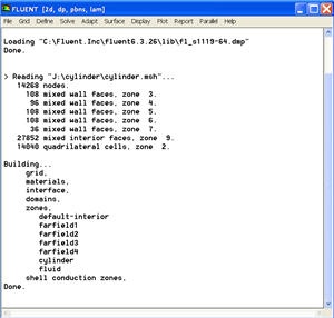
Navigate to the working directory and select the cylinder.msh file. This is the mesh file that was created using the preprocessor GAMBIT in the previous step. FLUENT reports the mesh statistics as it reads in the mesh:
| newwindow | ||||
|---|---|---|---|---|
| ||||
https://confluence.cornell.edu/download/attachments/103733026/step4_img001.jpg?version=1 |
Also, take a look under zones. We can see the five zones farfield1, farfield2, farfield3,farfield4, and cylinder that we defined in GAMBIT.
...
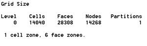
Main Menu > Grid > Info > Size
The following statistics info should appear (your number of cells might be slightly different because of slight different mesh criteria used):
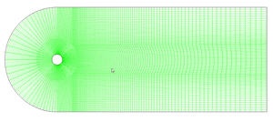
Display the grid:
Main Menu > Display > Grid...
Make sure all 5 6 items under Surfaces is selected. Then click Display. The graphics window opens and the grid is displayed in it. You can now click Close in the Grid Display menu to get back some desktop space. The graphics window will remain.Some of the operations available in the graphics window are:
| Info | ||
|---|---|---|
| ||
Translation: The grid can be translated in any direction by holding down the Left Mouse Button and then moving the mouse in the desired direction. |
Use these operations to zoom into the grid to obtain the view shown below.
| Warning | |
|---|---|
|
...
|
...
|
...
|
...
| newwindow | ||||
|---|---|---|---|---|
| ||||
https://confluence.cornell.edu/download/attachments/103733026/step4_img003.jpg?version=1 |
| Tip | ||
|---|---|---|
| ||
To get white background go to: |
You can also look at specific parts of the grid by choosing the boundaries you wish to view under Surfaces (click to select and click again to deselect a specific boundary). Click Display again when you have selected your boundaries. For example, the wall, outlet, and centerline boundaries have been selected in the following view:
These options will display the graph:
(Click picture for larger image)
For convenience, the button next to Surfaces selects all of the boundaries while the
deselects all of the boundaries at once.
Close the Grid Display Window when you are done.
Define Solver Properties
Main Menu > Define > Models > Solver
Choose Axisymmetric under Space. We'll use the defaults of pressure based ("segregated", in older versions) solver, implicit formulation, steady flow and absolute velocity formulation. Click OK.
Use the default setting. Click Cancel.
Main Menu > Define > Models > Viscous
Laminar flow is the default. So we don't need to change anything in this menu. Click Cancel.
Main Menu > Define > Models > Energy
For incompressible flow, the energy equation is decoupled from the continuity and momentum equations. We need to solve the energy equation only if we are interested in determining the temperature distribution. We will not deal with temperature in this example. So leave the Energy Equation unselected and click Cancel to exit the menu.
Define Material Properties
Main Menu > Define > Materials...
Change Density to 1.0 and Viscosity to 2e-3 0.1. These are the values that we specified under Problem Specification. We'll take both as constant.
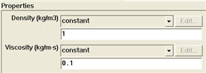
Click Change/Create. Close the window.
Define Operating Conditions
...
For all flows, FLUENT uses gauge pressure internally. Any time an absolute pressure is needed, it is generated by adding the operating pressure to the gauge pressure. We'll use the default value of 1 atm (101,325 Pa) as the Operating Pressure.
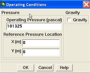
Click Cancel to leave the default in place.
Define Boundary Conditions
We'll now set the value of the velocity at the inlet and pressure at the outlet.
Use the following table to set boundary type of each zone.
Zone | Type |
farfield1 | velocity-inlet, V x = 1 m/s |
farfield2 | velocity-inlet, V x = 1 m/s |
farfield3 | velocity-inlet, V x = 1 m/s |
farfield4 | pressure-outlet |
cylinder | wall |
Main Menu > Define > Boundary Conditions...
We note here that the four types of boundaries we defined are specified as zones on the left side of the Boundary Conditions Window. The centerline zone should be selected by default. Make sure it is, then make sure the Type of this boundary is selected as axis and click Set.... Notice that there is nothing to set for the axis. Click OK.
Move down the list and select inlet under Zone. Note that FLUENT indicates that the Type of this boundary is velocity-inlet. Recall that the boundary type for the "inlet" was set in GAMBIT. If necessary, we can change the boundary type set previously in GAMBIT in this menu by selecting a different type from the list on the right.
Click on Set.... Enter 1 for Velocity Magnitude. Click OK. This sets the velocity of the fluid entering at the left boundary.
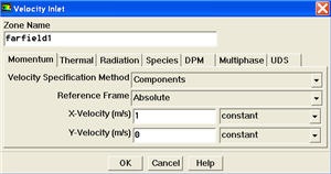
Select farfield1 under Zone. Change the Type of boundary as velocity-inlet. A new window will pop up. Change Magnitude, Normal to Boundary to Components under Velocity Specification Method. Input value 1 next to X-Velocity. Click OK. Do the same for farfield2 and farfield3.
The (absolute) pressure at the outlet farfield downstream is 1 atm. Since the operating pressure is set to 1 atm, the outlet gauge pressure = outlet absolute pressure - operating pressure = 0. Choose outlet farfield4 under Zone. The Type of this boundary is pressure-outlet. Click on Set.... The default value of the Gauge Pressure is 0. Click Cancel to leave the default in place.
Lastly, click on wall cylinder under Zones and make sure Type is set as wall. Click on each of the tabs and note that only momentum can be changed under the current conditions. This will not be so under later exercises so make a note of the location of these options. Click OK.
Click Close to close the Boundary Conditions menu.
Go to Step 5: Solve!
See and rate the complete Learning Module
...