 Sign-up for free online course on ANSYS simulations!
...
We'll next plot the velocity at the outlet as a function of the distance from the center of the pipe. To do this, we have to set the y axis of the graph to be the y axis of the pipe (the radial direction).
#plottingTo plot the position variable on the y axis of the graph, uncheck Position on X Axis under Options and choose Position on Y Axis instead. To make the position variable the radial distance from the centerline, under Plot Direction, change X to 0 and Y to 1. To plot the axial velocity on the x axis of the graph, for X Axis Function, pick Velocity... and Axial Velocity under that.
...
Now we can plot the velocity profiles at x=0.6m (x/D=3) and x=0.12m (x/D=6) along with the outlet profile. In the Solution XY plot menu, use the same settings as above. Under Surfaces, in addition to outlet, select line1 and line2. Make sure Node Values is selected under Options. Click Plot. Your symbols might be different from the ones below. You can change the symbols and line styles under the Curves... button. Click on Help in the Curves menu if you have problems figuring out how to change these settings.
...
One can plot vectors in the entire domain, or on selected surfaces. Let us plot the velocity vectors for the entire domain to see how the flow develops downstream of the inlet.
Main Menu > Display > Vectors... > Display
Zoom into the region near the inlet. (Click here to review the zoom functionality discussion in step 4.) The length and color of the arrows represent the velocity magnitude. The vector display is more intelligible if one makes the arrows shorter as follows: Change Scale to 0.4 in the Vectors menu and click Display.
You can reflect the plot about the axis to get an expanded sectional view:
Main Menu > Display > Views...
Under Mirror Planes, only the axis surface is listed since that is the only symmetry boundary in the present case. Select axis and click Apply. Close the Views window.
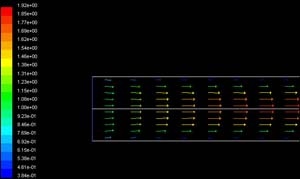
The velocity vectors provide a picture of how the flow develops downstream of the inlet. As the boundary layer grows, the flow near the wall is retarded by viscous friction. Note the sloping arrows in the near wall region close to the inlet. This indicates that the slowing of the flow in the near-wall region results in an injection of fluid into the region away from the wall to satisfy mass conservation. Thus, the velocity outside the boundary layer increases.
| Panel |
|---|
By default, one vector is drawn at the center of each cell. This can be seen by turning on the grid in the vector plot: Select Draw Grid in the Vectors menu and then click Display in the Grid Display as well as the Vectors menus. Velocity vectors are the default, but you can also plot other vector quantities. See section 27.1.3 of the user manual for more details about the vector plot functionality. |
Go to Step 7: Refine Mesh
See and rate the complete Learning Module
...