 Sign-up for free online course on ANSYS simulations!
...
We'll plot the variation of the axial velocity along the centerline.
Main Menu > Plot > XY Plot...
Make sure that Position on X Axis is set under Options, and X is set to 1 and Y to 0 under Plot Direction. This tells FLUENT to plot the x-coordinate value on the abscissa of the graph.
Under Y Axis Function, pick Velocity... and then in the box under that, pick Axial Velocity.
Please note that X Axis Function and Y Axis Function describe the x and y axes of the graph, which should not be confused with the x and y directions of the pipe.
Finally, select centerline under Surfaces since we are plotting the axial velocity along the centerline. This finishes setting up the plotting parameters.
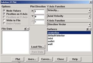
Click Plot.
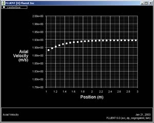
This brings up a plot of the axial velocity as a function of the distance along the centerline of the pipe.
...
Change the axes extents: In the Solution XY Plot window, click on Axes.... Under Options, deselect Auto Range. The boxes under Range should now be activated. Select X under Axis. Enter 1 for Minimum and 3 for Maximum under Range.
We'll turn on the grid lines to help estimate where the flow becomes fully developed. Check the boxes next to Major Rules and Minor Rules under Options. Click Apply.
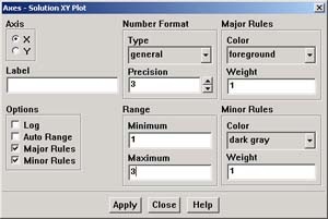
Now, pick Y under Axis and once again deselect Auto Range under Options, then enter 1.8 for Minimum and 2.0 for Maximum under Range. Also select Major Rules and Minor Rules to turn on the grid lines in the Y direction. We have now finished specifying the range for each axes, so click Apply and then Close.
Go back to the Solution XY Plot menu and click Plot to replot the graph with the new axes extents. We can see that the fully-developed region starts at around x=_3m and the centerline velocity in this region is _1.93 m/s.
...
In the Solution XY Plot Window, check the Write to File box under Options. The Plot button should have changed to Write.... Click on Write.... Enter vel.xy as the XY File Name and click OK. Check that this file has been created in your FLUENT working directory.
...
Leave the Solution XY Plot Window and the Graphics Window open and in the main FLUENT window click on:
File > Hardcopy ...
Under Format, choose one of the following three options:
EPS - if you have a postscript viewer, this is the best choice. EPS allows you to save the file in vector mode, which will offer the best viewable image quality. After selecting EPS, choose Vector from under File Type.
TIFF - this will offer a high resolution image of your graph. However, the image file generated will be rather large, so this is not recommended if you do not have a lot of room on your storage device.
JPG - this is small in size and viewable from all browsers. However, the quality of the image is not particularly good.
After selecting your desired image format and associated options, click on Save...
Enter vel.eps, vel.tif, or vel.jpg depending on your format choice and click OK.
Verify that the image file has been created in your working directory. You can now copy this file onto a disk or print it out for your records.
...
FLUENT provides a large amount of useful information in the online help that comes with the software. Let's probe the online help for information on calculating the coefficient of skin friction.
Main Menu > Help > User's Guide Index...
Click on S in the links on top and scroll down to skin friction coefficient. Click on the second 965 link (normally, you would have to go through each of the links until you find what you are looking for). We can see an excerpt on the skin coefficient as well as the equation for calculating it.
Click on the link for Reference Values panel, which tells us how to set the reference values used in calculating the skin coefficient.
...
Set the reference values:
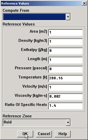
Main Menu > Report > Reference Values...
Select inlet under Compute From to tell FLUENT to calculate the reference values from the values at inlet. Check that density is 1 kg/m3 and velocity is 1 m/s. (Alternately, you could have just typed in the appropriate values). Click OK.
Go back to the Solution XY Plot menu. Uncheck Write to File under Options since we want to plot to the window right now. We can leave the other Options and Plot Direction as is since we are still plotting against the x distance along the pipe.
Under the Y Axis Function, pick Wall Fluxes..., and then Skin Friction Coefficient in the box under that.
Under Surfaces, select wall and unselect centerline by clicking on them.
Reset axes ranges: Go to Axes... and re-select Auto-Range for the Y axis. Click Apply. Set the range of the X axis from 1 to 8 by selecting X under Axis, entering 1 under Minimum, and 8 under Maximum in the Range box (remember to de-select Auto RangeAuto-Range first if it is checked).
Click Apply, Close, and then Plot in the Solution XY Plot Window.
...
Save the data from this plot: Pick Write to File under Options and click Write.... Enter cf.xy for XY File and click OK.
Velocity Profile
We'll next plot the velocity at the outlet as a function of the distance from the center of the pipe. To do this, we have to set the y axis of the graph to be the y axis of the pipe (the radial direction).
To plot the position variable on the y axis of the graph, uncheck Position on X Axis under Options and choose Position on Y Axis instead. To make the position variable the radial distance from the centerline, under Plot Direction, change X to 0 and Y to 1. To plot the axial velocity on the x axis of the graph, for X Axis Function, pick Velocity... and Axial Velocity under that.
...