 Sign-up for free online course on ANSYS simulations!
...
Finally, select centerline under Surfaces since we are plotting the axial velocity along the centerline. This finishes setting up the plotting parameters.
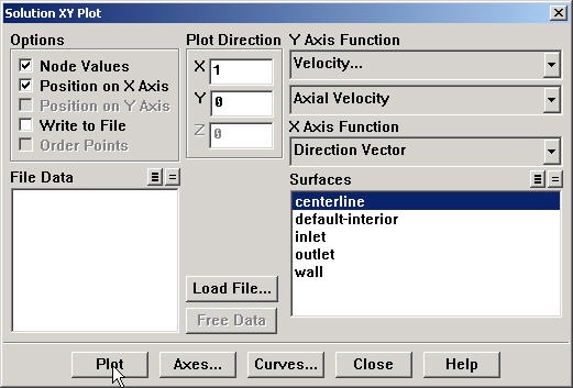
Click Plot.
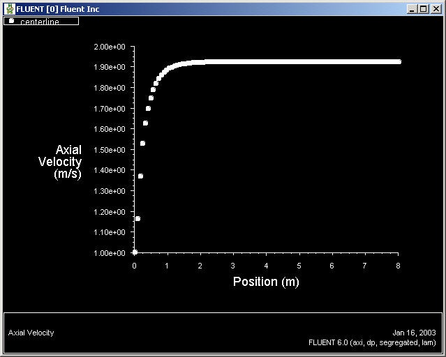
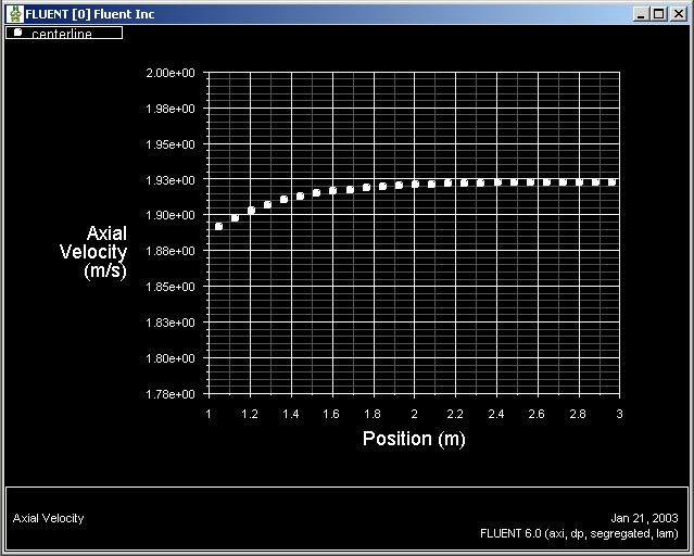
This brings up a plot of the axial velocity as a function of the distance along the centerline of the pipe.

(Click picture here for larger image)
In the graph that comes up, we can see that the velocity reaches a constant value beyond a certain distance from the inlet. This is the fully-developed flow region.
...
We'll turn on the grid lines to help estimate where the flow becomes fully developed. Check the boxes next to Major Rules and Minor Rules under Options. Click Apply.
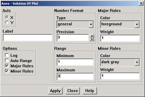
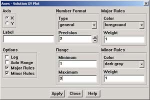
Now, pick Y under Axis and once again deselect Auto Range under Options, then enter 1.8 for Minimum and 2.0 for Maximum under Range. Also select Major Rules and Minor Rules to turn on the grid lines in the Y direction. We have now finished specifying the range for each axes, so click Apply and then Close.
Go back to the Solution XY Plot menu and click Plot to replot the graph with the new axes extents. We can see that the fully-developed region starts at around x=_3m and the centerline velocity in this region is _1.93 m/s.
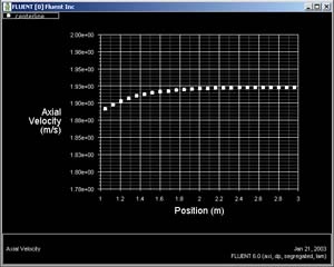
(Click picture here for larger image)
Saving the Plot
Save the data from this plot:
...
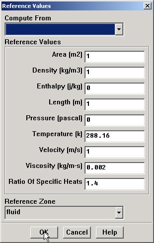
Select inlet under Compute From to tell FLUENT to calculate the reference values from the values at inlet. Check that density is 1 kg/m3 and velocity is 1 m/s. (Alternately, you could have just typed in the appropriate values). Click OK.
Go back to the Solution XY Plot menu. Uncheck Write to File under Options since we want to plot to the window right now. We can leave the other Options and Plot Direction as is since we are still plotting against the x distance along the pipe.
...
Click Apply, Close, and then Plot in the Solution XY Plot Window.
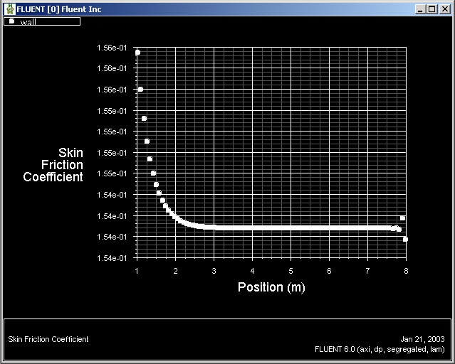
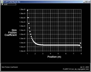
(Click picture here for larger image)
We can see that the fully developed region is reached at around x=3.0m and the skin friction coefficient in this region is around 1.54. Compare the numerical value of 1.54 with the theoretical, fully-developed value of 0.16.
...
Uncheck Write to File under Options so that we can see the graph. Click Plot.
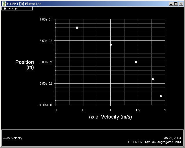
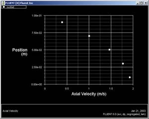
(Click picture here for larger image)
Does this look like a parabolic profile?
...
Under Mirror Planes, only the axis surface is listed since that is the only symmetry boundary in the present case. Select axis and click Apply. Close the Views window.
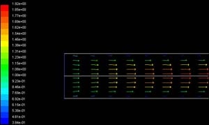
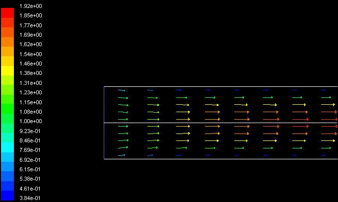
The velocity vectors provide a picture of how the flow develops downstream of the inlet. As the boundary layer grows, the flow near the wall is retarded by viscous friction. Note the sloping arrows in the near wall region close to the inlet. This indicates that the slowing of the flow in the near-wall region results in an injection of fluid into the region away from the wall to satisfy mass conservation. Thus, the velocity outside the boundary layer increases.
...