Page History

...

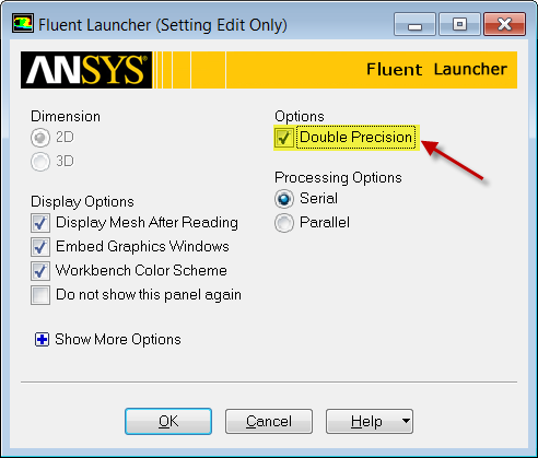
When the FLUENT Launcher appears change options to "Double Precision", and then click OK as shown below.The Double Precision option is used to select the double-precision solver. In the double-precision solver, each floating point number is represented using 64 bits in contrast to the single-precision solver which uses 32 bits. The extra bits increase not only the precision, but also the range of magnitudes that can be represented. The downside of using double precision is that it requires more memory.



Twiddle your thumbs a bit while the FLUENT interface starts up. This is where we'll specify the governing equations and boundary conditions for our boundary-value problem. On the left-hand side of the FLUENT interface, we see various items listed under Problem Setup. We will work from top to bottom of the Problem Setup items to setup the physics of our boundary-value problem. On the right hand side, we have the Graphics pane and, below that, the Command pane.

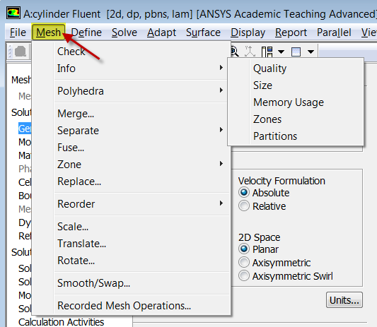
Check Mesh

(Click) Mesh > Info > Size
You should now have an output in the command pane stating that there are 18,432 cells.



(Click) Check > Perform Mesh > Check
You should see no errors in the command pane.

...

Note that pressures in the FLUENT interface are specified in terms of gauge values where:  gauge pressure = absolute pressure - reference pressure.  The reference pressure is 1 atm by default. So in our case the gauge pressure at the outlet is 0 atm which is also the default. The following video from the laminar pipe flow module in our MOOC free online course explains the advantages of working in terms of gauge pressures. The video discusses this in the context of laminar pipe flow but the same ideas apply for our cylinder flow too.  

...