 Sign-up for free online course on ANSYS simulations!
| Include Page | ||||
|---|---|---|---|---|
|
| Include Page | ||||
|---|---|---|---|---|
|
| Info | ||
|---|---|---|
| ||
Click here for the FLUENT 6.3.26 version. |
Numerical Results
Note that the results below are for a pipe of length 8 m. If your geometry was originally created from the laminar pipe tutorial from Dr. Bhaskaran's edX course, your pipe length will be 3 m. This is fine. The two lengths produce similar results since the flow becomes fully-developed before a distance of 3 m from the inlet.
After the solution is complete, close the FLUENT window to return to the Workbench window. Double click Results in the main Workbench window to open CFD Post, where we will be viewing the results. For a basic orientation on how to use CFD Post, pl. see the videos in the results step of the Laminar Pipe Flow tutorial.
The following instructions show only how to view results using the "chart" option. But one should really start by viewing velocity vectors, velocity/pressure/TKE contours etc. and check that the solution looks basically right. The Laminar Pipe Flow tutorial walks you through the steps to view vectors and contours in CFD Post.
...
Before viewing the results, we need to define the locations in CFD Post where we would like to view the results, namely the wall, centerline, and outlet.
Insert > Location > Line
Rename this location "Pipe Wall". Avoid naming locations in CFD Post with identical names to those used in FLUENT, this can cause problems. We will define the line by two points. Enter (0,0.1,0) for Point 1 and (8,0.1,0) for Point 2. Change Samples to 100.
Repeat the process for the two other locations needed:
| HTML Table |
|---|
Name | Point 1 | Point 2 |
"Pipe Centerline" | (0,0,0) | (8,0,0) |
"Pipe Outlet" | (8,0,0) | (8,0.1,0) |
y+
Turbulent flows are significantly affected by the presence of walls. The k-epsilon turbulence model is primarily valid away from walls and special treatment is required to make it valid near walls. The near-wall model is sensitive to the grid resolution which is assessed in the wall unit y+(defined in section 10.9.1 of the FLUENT user manual). We'll gloss over the details for now and use the following rule of thumb: select the near-wall resolution such that y+ > 30 or < 5 for the wall-adjacent cell when using the Enhanced Wall Treatment option. Look at section 10.9, Grid Considerations for Turbulent Flow Simulations, for details.
Let's plot y+ values for wall-adjacent cells to check how it compares with the recommendation mentioned above.
Insert > Chart
Let's rename the graph "Wall Y plus". Also, change Title to "Wall Y plus".
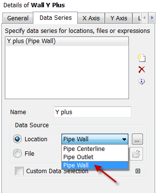
Data Series Tab
Rename the data series to "Y plus". Next, change Location to Pipe Wall.
X Axis Tab
Change Variable to X.
...
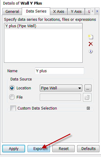
Export the data to a .csv file ("comma separated values") by clicking on Export. This file can be opened in Excel.
Centerline Velocity
Next, we would like to make a graph of the axial velocity along the centerline. We will do this by creating another chart.
...
To create a nondimensional version of the velocity profile, we first create a variable for r/D as shown in the the following video.
| HTML |
|---|
| Wiki Markup |
{html}<iframe width="600" height="338" src="//www.youtube.com/embed/aPYB_YZXeYs" frameborder="0" allowfullscreen></iframe>{html} |
Summary of the above video:
- In the right preview window, select Chart Viewer (Outlet Velocity selected in the tree)
- Go to Expressions tab in the same row as Outline
- Right click Expressions > New
- Name "r nondim exp"
- For Definition
- Right click > Variables > Y
- Insert /0.2[m] after Y
- Apply
- Go to Variables tab next to Outline
- Right click on Derived > New
- Name it r nondim
- For Expression, select "r nondim exp"
Then we make a plot of r/D vs. u/U using the steps shown below.
| HTML |
|---|
| Wiki Markup |
{html} <iframe width="600" height="450" src="//www.youtube.com/embed/QkAfGyxeXlo" frameborder="0" allowfullscreen></iframe> {html} |
Summary of the above video:
- Go to Outline tab
- Highlight Outlet Velocity Chart > Right click > Duplicate
- Name it Outlet Velocity nondim
- Go to Chart Viewer in the right preview
- Double click on Outlet Velocity nondim to ensure you are editing this new version
- Click on the Y Axis
- Select Variable r nondim
- Apply
The axis labels and legend can be modified as shown below.
| HTML |
|---|
| Wiki Markup |
{html} <iframe width="600" height="338" src="//www.youtube.com/embed/Nk3sXL_bSBo" frameborder="0" allowfullscreen></iframe> {html} |
Summary of the above video:
- In the General Table
- For Title, enter Nondimensional Velocity Profile
- Apply
- In the X Axis
- Scroll down and uncheck Use data for axis labels
- Enter in Custom Label u/U
- In the Y Axis
- Scroll down and uncheck Use data for axis labels
- Enter in Custom Label r/D
- In the Line Display
- Double click on Series 1 (Pipe Outlet)
- Uncheck Use series name for legend name
- Rename to Re = 10,000
We add the corresponding laminar profile. The necessary csv file can be downloaded here.
| HTML |
|---|
| Wiki Markup |
{html} <iframe width="600" height="450" src="//www.youtube.com/embed/y2GsRs2Pfio" frameborder="0" allowfullscreen></iframe> {html} |
Summary of the above video:
- Make sure you are editing Outlet Velocity nondim by double clicking on it
- Go to Data Series tab
- In the white space, right click > New
- Click File
- Select csv file downloaded from webpage
- Apply
- Go to Line Display
- Double click on the second curve
- Uncheck Use series name for legend name
- Name the Legend Name Laminar
- To save a copy of the chart, click on Save Picture icon in top toolbar
Non-dimensional Turbulent Viscosity Profile
| HTML |
|---|
| Wiki Markup |
{html} <iframe width="600" height="450" src="//www.youtube.com/embed/OEX1A8Q2tDw" frameborder="0" allowfullscreen></iframe> {html} |
Summary of the above video:
- Start FLUENT
- Go to File > Data File Quatntities
- Make sure Turbulent Velocity is selected, press OK
- Go back to FLUENT, click on Run Calculation
- Enter 1 in Number of Iterations
- Calculate
- Go back to Project Schematic
- Right click on Results > Refresh
- Go to CFD Post
- Click on Expressions tab
- Right click on Expressions > New
- Name it mut nondim exp
- In Definition white space:
- Right click > Variables > Eddy Viscosity
- Insert + 2e-5[kg/m/s]
- Divide whole thing by molecular viscosity 2e-5[kg/m/s]
- Apply
- Go to Variables tab
- Right click Derived > New
- Name it mut nondim
- Click Expression > select mut nondim exp
- Go to Outline > click on Chart icon in top toolbar
- Name it mut nondim plot
- Click on Data series
- Location Pipe Outlet
- Click on X Axis
- Variable mut nondim
- Click on Y Axis
- Variable r nondim
- Apply
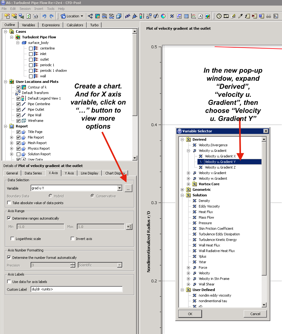
Tips on plotting additional derived quantities (such as velocity gradient)
In order to plot additional derived quantities such as the gradient, divergence or curl of the velocity field, you may find these quantities in a pop-up window in CFD post. Look at the illustration below for plotting velocity gradient in x.
Go to Step 7: Verification & Validation
...