 Sign-up for free online course on ANSYS simulations!
| Include Page | ||||
|---|---|---|---|---|
|
| Include Page | ||||
|---|---|---|---|---|
|
Verification and Validation
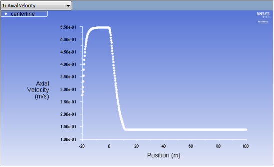
It is very important that you take the time to check the validity of your solution. Based on the velocity profile along the centerline, it can be seen that the max axis velocity in the small pipe is about 5.25e-1 m/s. However, in a full-developed laminar pipe flow, the analytical max axis velocity should be two times of the uniform inlet velocity, that is 5.54e-1 m/s. In other words, the results with the previous mesh are not good enough.
Refine Mesh
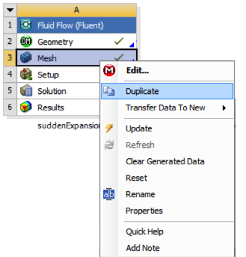
Let's repeat the solution on a finer mesh. For the finer mesh, the numbers of radial divisions will be twice as many as those used before. In the Workbench Project Page right click on Mesh then click Duplicate as shown below.
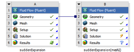
Rename the duplicate project to suddenExpansion (mesh2). You should have the following two projects in your Workbench Project Page.
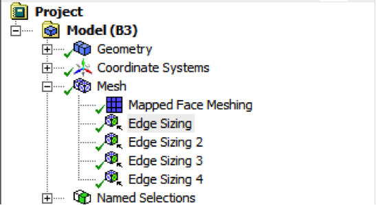
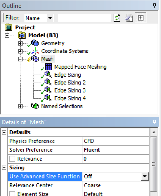
Next, double click on the Mesh cell of the suddenExpansion (mesh2) project. A new ANSYS Mesher window will open. Under Outline, expand Mesh and click on Edge Sizing, as shown below.
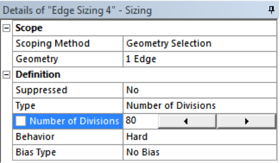
Here we will increase the numbers of cells in the radial direction. You may have different names of sizings. In my case, the "Edge Sizing" corresponds to the AB and EF edges, and “Edge Sizing 4” corresponds to the CD edge. Double the Number of Divisions of “Edge Sizing”
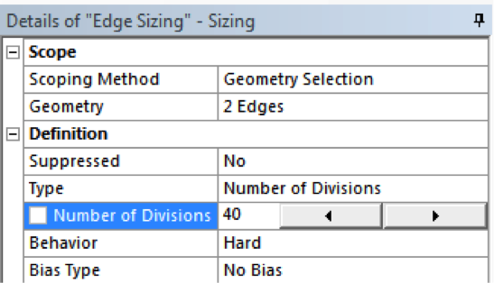
and “Edge Sizing 4”
Sometimes, you need to turn-off "Advanced Size Function" under "Details of Mesh" to get the mesher to accept the modified settings. That way the Advanced Size Function feature will not over-ride your settings (this feature is useful for meshing complex geometries). Click Mesh in the tree and turn off Advanced Size Function under "Details of Mesh" as shown below.
Then, click Update to generate the new mesh.

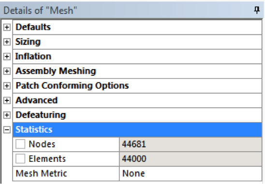
The mesh should now have 44000 elements. A quick glance of the mesh statistics reveals that there are indeed 44000 elements.
Compute the Solution
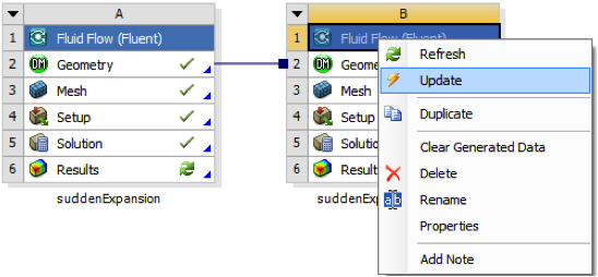
Close the ANSYS Mesher to go back to the Workbench Project Page. Under suddenExpansion (mesh2), right click on Fluid Flow (FLUENT) and click on Update, as shown below.
Now, wait a few minutes for FLUENT to obtain the solution for the refined mesh. After FLUENT obtains the solution, save your project.
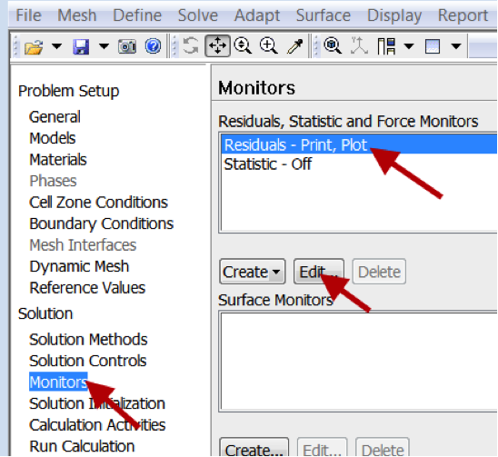
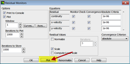
It is necessary to check that the solution iterations have converged. Launch FLUENT by double clicking on Solution of the "suddenExpansion (mesh2)" project in the Workbench Project Page. After FLUENT launches, select Monitors > Residuals > Edit... and then Plot, as shown in the images below.
If the solution hasn't converged, one needs to run more iterations by selecting Run Calculation. You may want to increase the number of iterations. Ensure that you have a converged solution and save the project. Then, if you double-click on Results for mesh2 in the project page, you'll see that all results have been updated for the new mesh.
Velocity profile
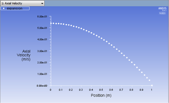
The plot below shows the profile of the axial velocity along the centerline (y = 0 m) with the refined mesh. It can be seen that the max velocity in the small pipe is about 5.50e-1 m/s, which is close to the analytical solution (5.54e-1 m/s) and better than that of the previous mesh.
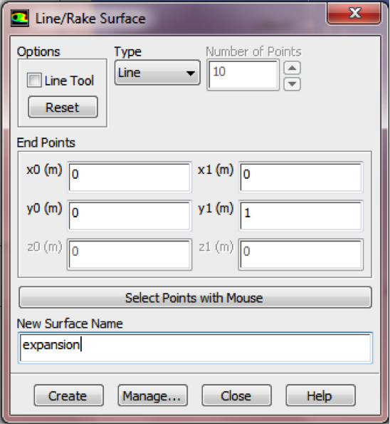
Here we will create a straight line for the expansion entrance, which is from (x0, y0) = (0, 0) to (x1, y1) = (0, 1). Select Line under Surface. Enter x0 = 0, y0 = 0, x1 = 0, y1 = 1. Enter expansion under New Surface Name. Click Create.
Then, plot the velocity profile along the expansion line. In the Solution XY Plot menu make sure that Position on X Axis is selected, and X is set to 0 and Y is set to 1.
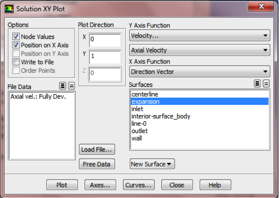
Then, click Plot and you should obtain the following output.
You can also plot axial velocity profiles at x = 1 m, 2 m, 3 m, 4 m, 5 m and 6 m as shown below. The numbers of the lines also indicate the distances from the expansion entrance to these lines.
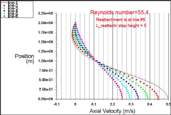
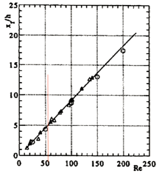
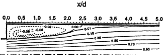
As you can see from the velocity profiles, the end of the recirculation region is at x = 5 m. In other words, the recirculation length for Re = 55.4 is about 5 times of the inlet radius, which agree well with the experimental data (Hammad et al., Experiments in Fluids, 1999, 26:266-271) shown below.
Streamline
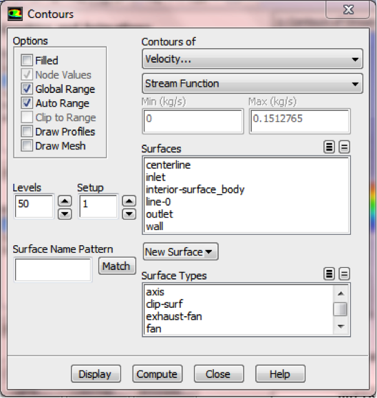
First, click on Graphics & Animations. Next, double click on Contours which is located under Graphics. Select Velocity and Stream Function under Contours of, and change the number of Levels to 50, as shown below.
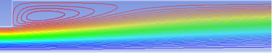
Then, click on Display. Zoom into the region near the expansion. The streamlines calculated with FLUENT are presented blow, and compared with the streamlines obtained via PIV experiment (Hammad et al., Experiments in Fluids, 1999, 26:266-271). It can be seen that the numerical result agree with the experiment one.
For more strict comparison, one should export the results from FLUENT, re-plot it in TECPLOT or some other post-processing software, and compare the value of stream function, redevelopment length and recirculation length carefully. One can also increase the inlet velocity so that Re = 200, and then compare the results with experiment data presented in the reference.