Page History

...

Let's get FLUENT to solve our nonlinear BVP. It'll introduce discretization and linearization errors in the process, as discussed in the Pre-Analysis step. We'll check the level of numerical errors later in the Verification & validation step. There are lots of knobs in the Solution menu that you can twiddle to improve your numerical solution to the BVP. We'll not mess with most of these since the default settings yield an adequate numerical solution for our problem. We could get a slight improvement in accuracy by fiddling various knobs which we'll refrain from doing.

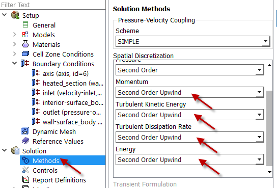
Solution > Solution Methods

The FLUENT solver converts our BVP to a set of algebraic equations through a process called discretization. We'll use second-order discretization for which the error is of the order of the square of the mesh spacing. This is more accurate (albeit less stable) than first-order discretization where the error is of the order of the mesh spacing.  Choose Second-Order Upwind for all equations as shown below.

Image RemovedImage Added

To set the convergence criterion identified in the flowchart above , select:

Solution > Monitors > ResidualsResidual

We see that we need to provide a convergence criterion for each PDE that is being solved. The solver will stop iterating when mass, momentum, energy, k and epsilon imbalances (called residuals) fall below the convergence tolerance. We'll use a residual tolerance of 10^-6 for all six PDE's being solved. FLUENT will consider the iterations have converged when all six residuals have fallen below this tolerance. Set the residuals tolerance as shown in the figure below. Make sure to scroll down and set the tolerance for k and epsilon equations also. 

Image Modified

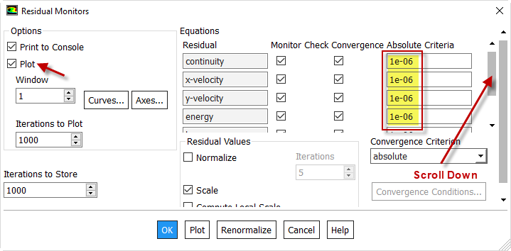
Also make sure Plot box is checked as shown above. This will help you monitor how/whether the solution is proceeding to convergence as the iterations are carried out. Click OK.

Next, we set the initial guess indicated in the flowchart. The initial guess can be entered using:

Solution > Solution Initialization

We need to provide FLUENT with an initial guess for the flow variables (velocity, pressure etc.) to start the iterations. For this example, we know the conditions at the inlet of the pipe (except for pressure which is set to zero gauge by default). Initialize the entire flowfield to the specified values at the inlet: First, select Standard Initialization, then under Compute from, select Inlet and click Initialize.

...