 Sign-up for free online course on ANSYS simulations!
...
| Panel |
|---|
Author: Rajesh Bhaskaran & Yong Sheng Khoo, Cornell University Problem Specification |
...
Display > Graphics and Animations > Vectors > Set up...
Select Velocity under Vectors of and Velocity... under Color by. Set Scale to 0.4
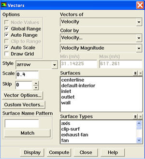
Click Display.
step6_2.png
We see that the flow is smoothly accelerating from subsonic to supersonic.
| Info | ||
|---|---|---|
| ||
Display > Views... |
| Info | ||
|---|---|---|
| ||
To get white background go to: Click Preview. Click No when prompted "Reset graphics window?" |
...
Let's look at how pressure changes in the nozzle.
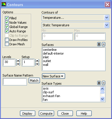
Display > Graphics and Animations > Contours > Set up
Select Pressure... and Static Pressure under Contours of. Use Levels of 30
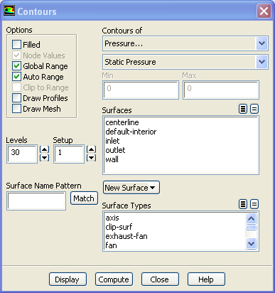
Click Display.
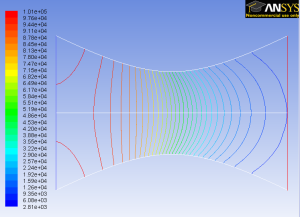
Notice that the pressure decreases as it flows to the right.
...
Let's look at the total pressure in the nozzle
Display > Graphics and Animations > Contours
Select Pressure... and Total Pressure under Contours of. Select Filled. Use Levels of 100.
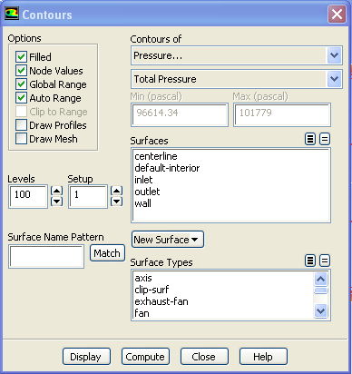
Click Display.
Around the nozzle outlet, we see that there is a pressure loss because of the numerical dissipation.
...
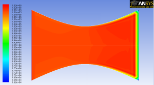
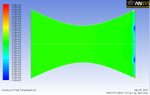
Let's investigate or verify the temperature properties in the nozzle.
Display > Graphics and Animations > Contours
Select Temperature... and Static Temperature under Contours of. Use Levels of 30.
Click Display.
As we can see, the temperature decreases from left to right in the nozzle, indicating a transfer of internal energy to kinetic energy as the fluid speeds up.
...
Now let's look at the total pressure in the nozzle
Display > Graphics and Animations > Contours
Select Temperature.. .and Total Temperature under Contours of. Select Filled. Use Levels of 100.
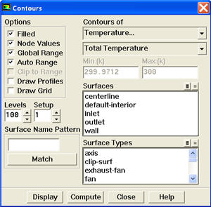
Click Display.
Looking at the scale, we see that the total temperature is uniform 300 K throughout the nozzle. The contour abnormality at the outlet of the nozzle is due to the round off errors.
...
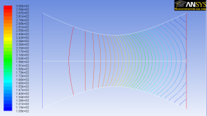
Let's now look at the Mach number
Display > Contours
Select Velocity...under Contours of and select Mach Number. Set Levels to 30.
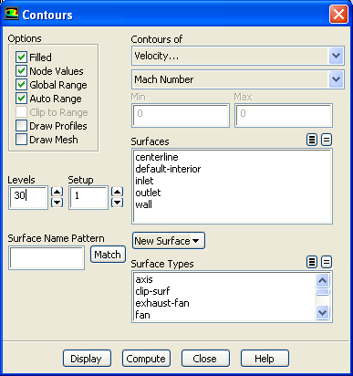
Click Display.
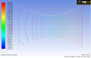
For 1D case, mach number is a function of x position. For 1D case, we are supposed to see vertical contour of mach numbers that are parallel to each other.
...
Let's look at the pressure along the centerline and the wall.
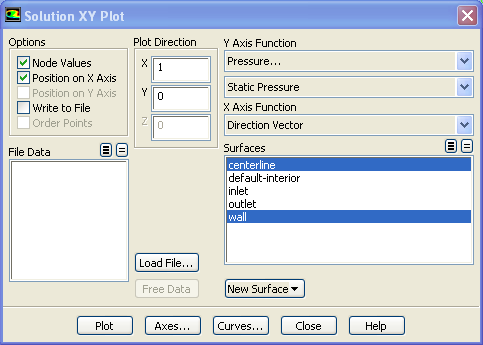
Under Results > Plots > XY Plot > Set up
Make sure that under Y-Axis Function, you see Pressure...and Static Pressure. Under Surfaces, select centerline and wall. Click Plot. By default FLUENT displays the plots using graphics but we will modify them to display lines which can be more helpful when analyzing the plot.
...
On the XY Plot window click on the Curves button. Change the Pattern to a line, Select a blank as a Symbol and change the Weight to any number greater than 2. To do this for multiple curves use the arrow buttons to navigate through the different curves displayed on the plot.
...
It is good to write the data into a file to have greater flexibility on how to present the result in the report. At the same XY Plot windows, select Write to File. Then click Write... Name the file "p.xy" in the directory that you prefer.
Open "p.xy" file with notepad or other word processing software. At the top, we see:
...
Let's plot the variation of Mach number in the axial direction at the axis and wall. In addition, we will plot the corresponding variation from 1D theory. You can download the file here: mach_1D.xy. This file is a text file. You can look at the format of this file by reading it into Wordpad.
Plot > XY Plot. Under the Y Axis Function, select Velocity... and Mach Number.
Also, since we are going to plot this number at both the wall and axis, select centerline and wall under Surfaces.
Then, load the mach_1D.xyby clicking on Load File....
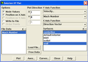
ClickPlot.
| Note | ||
|---|---|---|
| ||
The green line in the plot below SHOULD be in symbols. This will be corrected soon. |
...
Save this plot as machplot.xy by checking Write to File and clicking Write....
Go to Step 7: Verification & Validation
...