Page History

...

From these contours, you can observe that the air is being entrained near the jet inlet, and that the jet expands slightly along the x-direction. Also By knowing that the flow velocity is related to the stream function Ψ by u U = ∂Ψ/∂y and v V = - ∂Ψ/∂x, one can see that the stream functions function values will be smaller in the entrainment and jet stream areas, because the flow is more strongly linear there. 

Now go to 'Plots'-Results-Plots. Select XY Plot and make click "Set Up". Make a plot of how the axial velocity and half-width vary varies with axial distance x. These This plot and the half-width plot that you will create below can be used to examine the self similarity of the solution. 

To make the plot of the velocity variation along the centerline, adjust the XY plot dialogue box as shown below (in particular, adjust the plot direction to be values under Plot Direction so that the direction is along X):

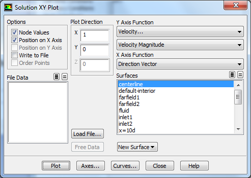
Click "Plot". This will give you the centerline plot:

...

To obtain the half width, export the X coordinate, Y coordinate, and Axial Velocity:

. Go to File-Export-Solution Data. Select 'X-coordinate', 'Y-coordinate', and 'Axial Velocity' as values to export. Export them along the centerline, and at various X locations (like surface X=10D) as an ASCII type file types. With the downloaded data, you can either copy it into Excel, or use write a short Matlab script and calling this function to read in ASCII files at the specified X locations (this is the easiest option!). 

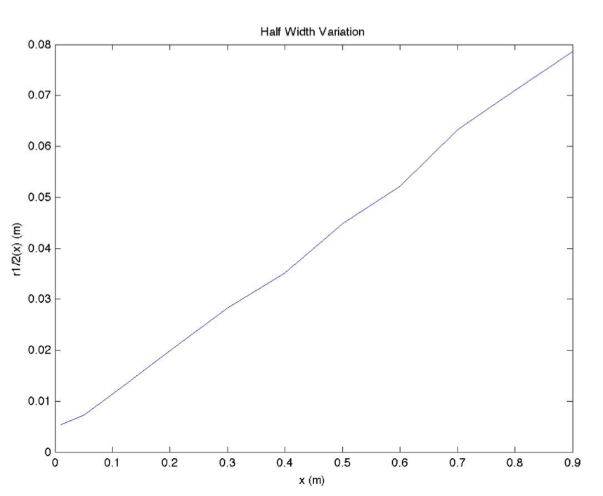
Using the Matlab script and plotting Y-coordinate approximate locations at which U=U_center/2 half width locations (determined by examining the values read in to Excel/Matlab to find the closest Y-coordinate at each X-location you exported at which U=U_center/2) gives the half width variation R(x)(1/2). The half width appears to increase approximately linearly along X. Keep these half width locations saved for future use.

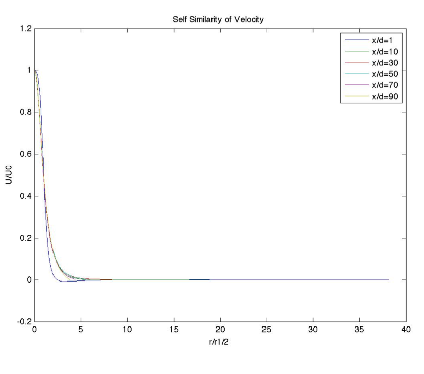
An additional step is to plot the self-similar profiles of the axial velocity U (scaled by the centerline velocity U_Center) vs radial distance (the Y-coordinate scaled by the half width R1/2(x) that you computed above) at various X locations, using the same exported data. The profiles appear to be self similar, although at X values closer to the inlet they will do not match exactly due to the additional entrainment effects.

Go to Step 4: Turbulent Jet Setup and Solution

...