| Include Page |
|---|
| FLUENT Google Analytics |
|---|
| FLUENT Google Analytics |
|---|
|
| Include Page |
|---|
| Flat Plate Boundary Layer - Panel |
|---|
| Flat Plate Boundary Layer - Panel |
|---|
|
Numerical Solution
| HTML |
|---|
<iframe width="560" height="315" src="https://www.youtube.com/embed/ctg-pEf397Q" frameborder="0" allow="accelerometer; autoplay; encrypted-media; gyroscope; picture-in-picture" allowfullscreen></iframe> |
Second Order Scheme
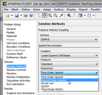
A second-order discretization scheme will be used to approximate the solution. In order to implement the second order scheme click on Solution Methods then click on Momentum and select Second Order Upwind as shown in the image below.
| newwindow |
|---|
| Click Here for Higher Resolution |
|---|
| Click Here for Higher Resolution |
|---|
|
https://confluence.cornell.edu/download/attachments/118771076/SecOrder_Full.png |
Set Convergence Criteria
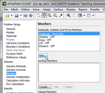
FLUENT reports a residual for each governing equation being solved. The residual is a measure of how well the current solution satisfies the discrete form of each governing equation. We'll iterate the solution until the residual for each equation falls below 1e-6. In order to specify the residual criteria (Click) Monitors > Residuals > Edit..., as shown in the image below.
| newwindow |
|---|
| Click Here for Higher Resolution |
|---|
| Click Here for Higher Resolution |
|---|
|
https://confluence.cornell.edu/download/attachments/118771076/EditResid_Full.png |
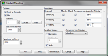
Next, change the residual under
Convergence Criterion for
continuity,
x-velocity,and
y-velocity, all to 1e-6, as can be seen below.
| newwindow |
|---|
| Click Here for Higher Resolution |
|---|
| Click Here for Higher Resolution |
|---|
|
https://confluence.cornell.edu/download/attachments/118771076/ResidMon_Full.png |
Lastly, click
OK to close the
Residual Monitors menu.
Set Initial Guess
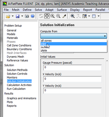
Here, the flow field will be initialized to the values at the inlet. That is, the initial values of all the cells will be set to 1 m/s and 0 Pa for x velocity and gauge pressure respectively. In order to carry out the initialization click on Solution Initialization then click on Compute from and select inlet as shown below.
| newwindow |
|---|
| Click Here for Higher Resolution |
|---|
| Click Here for Higher Resolution |
|---|
|
https://confluence.cornell.edu/download/attachments/118771076/CompFromInlet_Full.png |
Then, click the
Initialize button,

. This completes the initialization process.
Alternately, you could set the
Gauge Pressure to 0 and set the
X Velocity to 1 m/s as shown below.
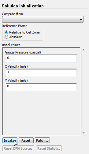
Then, you would need to press the
Initialize button to apply the specified initial values to all the cells. Either method will give you the same results.
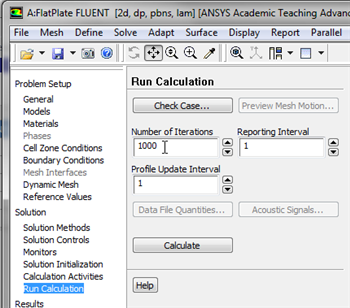
Iterate Until Convergence
Prior, to running the calculation the maximum number of iterations must be set. To specify the maximum number of iterations click on Run Calculation then set the Number of Iterations to 1000, as shown in the image below.
| newwindow |
|---|
| Click Here for Higher Resolution |
|---|
| Click Here for Higher Resolution |
|---|
|
https://confluence.cornell.edu/download/attachments/118771076/1kIter_Full.png |
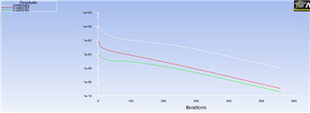
As a safeguard save the project now. Now, click on
Calculate two times in order to run the calculation. The residuals for each iteration are printed out as well as plotted in the graphics window as they are calculated. After running the calculation, you should obtain the following residual plot.
| newwindow |
|---|
| Click Here for Higher Resolution |
|---|
| Click Here for Higher Resolution |
|---|
|
https://confluence.cornell.edu/download/attachments/118771076/ResPlot_Full.png |
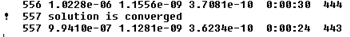
The residuals fall below the specified convergence criterion of 1e-6 in about 557 iterations, as shown below. Actual number of convergence steps may vary slightly.
| newwindow |
|---|
| Click Here for Higher Resolution |
|---|
| Click Here for Higher Resolution |
|---|
|
https://confluence.cornell.edu/download/attachments/118771076/SolConv_Full.png |
At this point, save the project once again.
Go to Step 6: Numerical ResultsGo to all FLUENT Learning Modules
 Sign-up for free online course on ANSYS simulations!