Page History

...

We'll use a second-order discretization scheme. Under Discretization, set Flow to Second Order Upwind. Under Solver Parameters, set the Courant Number to 0.1.

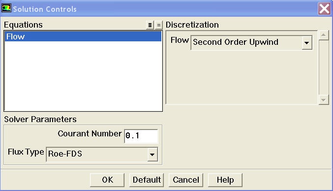
Click OK.

Solve > Initialize > Initialize...

This is where we set the initial guess values for the iterative solution. We'll use the farfield values (M=3, p=1 atm, T=300 K) as the initial guess for the entire flowfield. Select farfield under Compute From. This fills in values from the farfield boundary in the corresponding boxes. (Alternately, I could have typed in these values but I like to palm off as much grunt work as possible to the computer.)

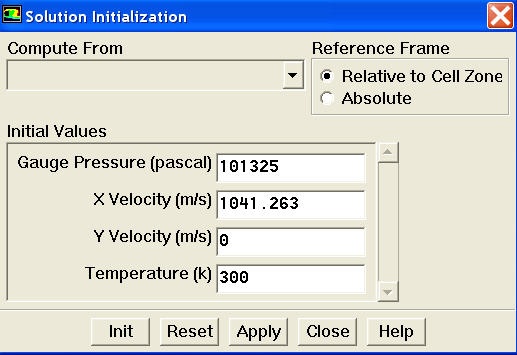
Click Init. Now, for each cell in the mesh, M=3, p=1 atm, T=300 K. These values will of course get updated as we iterate the solution below.

...

Solve > Monitors > Residual...

Set Absolute Criteria for all equations to 1e-6.

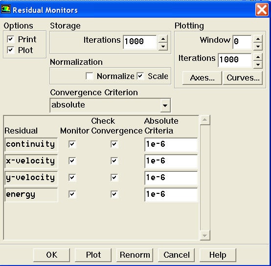
Also, under Options, select Plot. This will plot the residuals in the graphics window as they are calculated, giving you a visual feel for if/how the iterations are proceeding to convergence.

Click OK.

Main Menu > File > Write > Case...

This will save your FLUENT settings and the mesh to a "case" file. Type in wedge.cas for Case File. Click OK.

Solve > Iterate

Set the Number of Iterations to 1000. Click Iterate.

The residuals for each iteration are printed out as well as plotted in the graphics window as they are calculated. The residuals after 1000 iterations are not below the convergence criterion of 1e-6 specified before. So run the solution for 1000 more iterations. The solution converges in about 1510 iterations; the residuals for all the governing equations are below 1e-6 at this point.

...