Pre-Analysis & Start-Up

Pre-Analysis

In the Pre-Analysis step, we will review the following:

• Mathematical model: (e.g.: We will look at the governing equations, boundary conditions, and the assumptions contained within the mathematical model.)
• Numerical solution procedure in ANSYS: (e.g.: We will briefly overview the solution strategy used by ANSYS and contrast it to the hand calculation approach.)
• Hand-calculations of expected results: (e.g.: We will use an analytical solution of the mathematical model to predict the expected stress field from ANSYS. We will pay close attention to additional assumptions that have to be made in order to obtain an analytical solution.)

Mathematical Model 

Governing Equations

The governing equations solved here are conservation of mass and the conservation of momentum (Navier-Stokes equations), taken in a frame of reference moving with the turbine:

• Conservation of Mass:
  
• Navier-Stokes equations, simplified for constant angular velocity, in a moving frame of reference:
  
  where:
   and 

FLUENT will solve this in a moving frame of reference. This is a good simplification because with it we do not have to deal with a moving mesh. (yet! Keep checking for future tutorials on that!)

Note that we are solving a turbulent problem, and we will assume a k-epsilon model with default FLUENT values.

Boundary Conditions

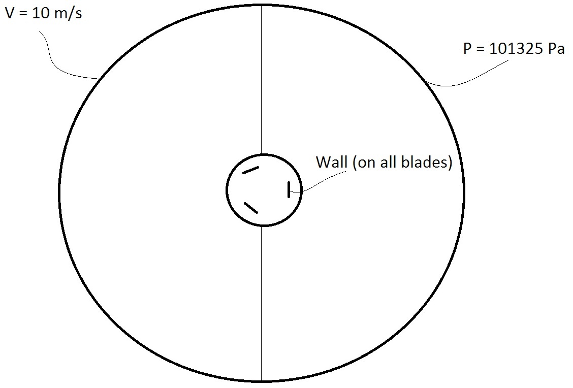
To solve this in FLUENT, we will need to create a region a few times larger than the main geometry of the turbine. This region is where the presence of the turbine disturbs the flow. This can be seen as the outer circle in the following figure. Note that we could have made any geometry for this "far-field" zone, but to simplify the boundaries a circle was chosen. 

The boundary conditions are:

• Inlet (far-field): constant velocity in the x-direction of 10m/s, with a turbulent intensity of 5% and a turbulent viscosity ratio of 1.
• Outlet (far-field): absolute pressure of 101325 Pa, or 1 atm.
• Blades: wall, so no velocity. (No-slip condition).

Numerical Solution Procedure in ANSYS

FLUENT will follow the Finite-Volume Method and will divide the domain into multiple control volumes or "cells".
From the integral form of the governing equations, FLUENT will perform a control volume balance for each cell and write nonlinear algebraic equations for them, and then linearize these equations.
Next, it will iteratively solve these equations and stop the iteration when the Residuals are below a certain specified tolerance.

Velocity, pressure, angular velocity and turbulence parameter k are calculated in the cell centers after inverting the matrix of the system of algebraic equations of cell-center values.
With these values, we will derive everything else that we might want, like wall shear, velocity field, etc. in the post-process step.

Hand-Calculations of Expected Results

Tip Speed Ratio (TSR)

The expression for TSR is: 

\begin{equation*}
\displaystyle \lambda = \frac{\textrm{Velocity at the blade tip}}{\textrm{Incoming wind velocity}} = \frac{r \times \omega_{}}{U}
\end{equation*}

Using r as the distance from the center to the mid point of a blade: r=0.04m.

The angular velocity is 40rpm which corresponds to 4.1888rad/s.

Therefore, the expected velocity at the center of the blades is 0.1676m/s and therefore the TSR is 0.01676.

We may want to use the following simplifications:

• Assume the airfoils are flat plates of dimension 0.1x2cm positioned on a pitch angle of 20deg, i.e. the plates are placed such that when they are at the upper-most part of its trajectory, they form an angle of 20deg with the horizontal.
• Incoming flow with a constant profile of 10m/s in the horizontal direction
• The downstream pressure is a constant at 101325 Pa.
• Air with a density of 1.225kg/m^3 and a viscosity of 1.7894e-5 Pa.s. 
• 2D analysis

Start-Up

Now we'll start with the Ansys part. It is recommended that you leave this tutorial side by side with the ANSYS screen, with ANSYS taking 2/3 of the screen and the tutorial, 1/3.

Start by opening ANSYS Workbench. 

If your screen does not look like this, you can click View > Reset Window Layout. 

Locate Fluid Flow (Fluent) under Analysis Systems on the left portion of the window. 

Click and hold the button down, and drag it into the Project Schematics, which is the central region of the screen. Note that a red rectangle will show up before you drag, indicating where you should "drop" the dragged item

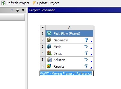
After releasing the click your window will look similar to this:

Rename the project to VAWT - Moving Frame of Reference

Now, Save your project by clicking File > Save and selecting the desired location and name.

Note: ANSYS creates two entities when saving: and .wbpj file and a folder. You will need to have both on the same directory in order to resume the project. It is possible to save it into a single file by going to File > Archive. This will generate a single .wbpz file, which is easier to move in case you're on a temporary directory.

Go to Step 2: Geometry

Go to all FLUENT Learning Modules