Sign-up for free online course on ANSYS simulations!
Unable to render {include} The included page could not be found.
Unable to render {include} The included page could not be found.
Unable to render {include} The included page could not be found.
Unable to render {include} The included page could not be found.
Step 4: Specify geometry
Since the geometry, material properties and loading are all symmetric with respect to the horizontal and vertical centerlines, we need to model only a quarter of the plate. We will take the origin of the coordinate system to be at the center of the hole and model only the top right quadrant. We'll create the geometry by creating a square area of side a and subtracting the circular sector of radius r from it.
Create the Square
Main Menu > Preprocessor > Modeling >Create > Areas >Rectangle > By Dimensions
X1 and X2 are the x-coordinates of the left and right edges of the square, respectively. Enter 0 for X1, a for X2.
Y1 and Y2 are the y-coordinates of the bottom and top edges of the square, respectively. Enter 0 for Y1, a for Y2.
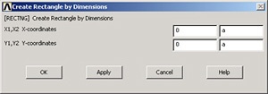
Click OK. You should see a square appear in the graphics window.
Create the Circular Sector
Main Menu > Preprocessor > Modeling > Create > Areas > Circle > Partial Annulus
WP X and WP Y are the x- and y-coordinates of the center of the circular arc. So enter 0 for both WP X and WP Y (WP refers to the Working Plane which by default coincides with the global Cartesian coordinate system. We won't have to worry about the working plane in this friendly example.)
Rad-1 is the radius of the inner circular arc. We want to create a solid rather than an annular arc. Enter 0 for Rad-1 to create a solid arc.
Rad-2 is the (outer) radius of the arc. Since we had defined the hole radius as parameter r earlier, enter r for Rad-2.
Theta-1 and Theta-2 are the starting and ending angles of the arc, respectively. These angles need to be specified in degrees. Enter 0 for Theta-1 and 90 for Theta-2. Click OK.
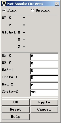
This will create and draw the circular sector. You'll see a white line denoting the circular sector.
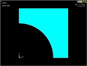
Subtract Circular Sector from Square
Main Menu > Preprocessor >Modeling > Operate > Booleans > Subtract > Areas
In the Input window, ANSYS tells you to "pick or enter base areas from which to subtract". So we pick the square area as follows: Hold down the left mouse button, move the cursor over the areas until the square is selected (it will change color) and release the left mouse button. Click OK.
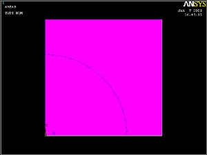
In the Input window, ANSYS now tells you to "pick or enter areas to be subtracted". So select the circular sector by holding down and releasing the left mouse button. Click OK.
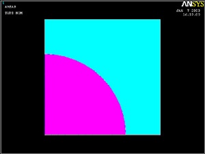
If you did this correctly, you will see that the circular sector has been subtracted out from the square area.
You can also select areas during the Boolean subtract operation by simply clicking on them but it becomes difficult to select areas (and other components) in this fashion in more complicated geometries. That's why I made you use the "holding-down-the-mouse-and-releasing" technique.
If you picked an area incorrectly, you can unpick it by clicking the right mouse button and selecting the area. The cursor changes to a downward arrow during an unpick operation. Right-click to return to pick mode.
Save Your Work
Toolbar > SAVE_DB
Step 5: Mesh geometry
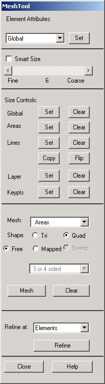
Bring up the MeshTool:
Main Menu > Preprocessor > Meshing > MeshTool
The MeshTool is used to control and generate the mesh.
Set Meshing Parameters
We'll now specify the element type, real constant set and material property set to be used in the meshing. Since we have only one of each, we can assign them to the entire geometry using the Global option under Element Attributes.
Make sure Global is selected under Element Attributes and click on Set.
This brings up the Meshing Attributes menu. You will see that the correct element type and material number are already selected since we have only one of each. Recall that no real constants need to be defined for PLANE42 element type with the plane stress keyoption.
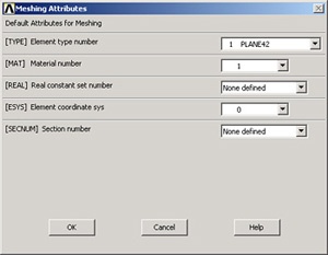
Click OK. ANSYS now knows what element type and material type to use for the mesh.
Set Mesh Size
Instead of setting the mesh size at each boundary, we'll use the SmartSize option which enables automatic element sizing. Click on the SmartSize checkbox so that a tickmark appears in it.
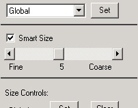
The only input necessary for the SmartSize option is the overall element size level for meshing. The element size level determines the fineness of the mesh. Its value is controlled by the slider shown in the above picture. Change the setting for the overall element size level to 5 by moving the slider under SmartSize to the left.
Mesh Areas
In the MeshTool, make sure Areas is selected in the drop-down list next to Mesh. This means the geometry components to be meshed are areas (as opposed to lines or volumes). We'll use quadrilateral elements. So make sure the default option of Quad is selected under Shape. We'll also use the default of Free meshing.
Click on the Mesh button. This brings up the pick menu.
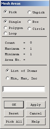
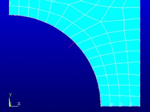
In the Input window, ANSYS tells you to "pick or enter areas to be meshed". Since we have only one area to be meshed, click on Pick All. The geometry has been meshed and the elements are plotted in the Graphics window. Close the MeshTool.
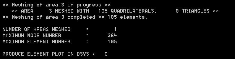
The mesh statistics are reported in the Output window (usually hiding behind the Graphics window):
** AREA 3 MESHED WITH 105 QUADRILATERALS, 0 TRIANGLES **
** Meshing of area 3 completed ** 105 elements.
NUMBER OF AREAS MESHED = 1
MAXIMUM NODE NUMBER = 130
MAXIMUM ELEMENT NUMBER = 105
Save Your Work
Toolbar > SAVE_DB
Go to Step 6: Specify boundary conditions
Step 6: Specify boundary conditions
Next, we step up to the plate to define the displacement constraints and loads. Recall that in ANSYS terminology, the displacement constraints are also "loads". As in the truss tutorial, we'll apply the loads to the geometry rather than the mesh. That way we won't have to reapply the loads on changing the mesh.
Apply Symmetry Boundary Conditions
ANSYS provides the option of applying a "symmetry boundary condition" along lines of symmetry.
Main Menu > Preprocessor > Loads > Define Loads > Apply > Structural > Displacement > Symmetry B.C. > On Lines
Select the straight lines corresponding to the left and bottom edges (which are the lines of symmetry for this problem) by clicking on them. Click OK in the pick menu. The symbol s appears along these lines indicating that the symmetry B.C. is applied along these lines.
Apply Pressure
Main Menu > Preprocessor > Loads > Define Loads > Apply > Structural > Pressure > On Lines
Select the circular arc and click OK. This brings up the Apply Pressure on Lines menu. Enter p for Value and click OK. A single red arrow denotes the pressure and the direction in which it is acting.
Check Loads
Let's check that the displacement constraints have been applied correctly.
Utility Menu > List > Loads > DOF constraints > On All Lines
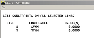
Symmetry BCs are applied on lines 8 and 9. Turn on line numbering:
Utility Menu > PlotCtrls > Numbering
Turn on Line numbers and click OK. Are lines L8 and L9 the ones on which you want the symmetry BCs?
Similarly, check that the pressure is applied correctly using Utility Menu > List > Loads > Surface Loads > On All Lines. Note that VALI and VALJ would be different if the applied pressure were linearly varying along the line.
Turn off line numbering: Utility Menu > PlotCtrls > Numbering. Turn off Line numbers and click OK.
Save Your Work
Toolbar > SAVE_DB
Step 7: Solve!
Enter solution module:
Main Menu > Solution
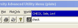
Enter check in the Input window and press Enter.
If the problem has been set up correctly, there will be no errors or warnings reported. If you look in the Output window, you should see the message: The analysis data was checked and no warnings or errors were found.
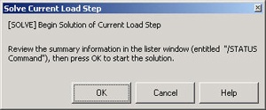
Main Menu > Solution > Solve > Current LS
Recall from the truss tutorial that this solves the current load step (LS) i. e. the current loading conditions. In this problem also, there is only one load step.
Review the information in the /STATUS Command window. Close this window.
Click OK in Solve Current Load Step menu.
ANSYS performs the solution and a window should pop up saying "Solution is done!". Congratulations! Close the window.
Verify that ANSYS has created a file called plate.rst in your working directory. This file contains the results of the (previous) solve.
Go to Step 8: Postprocess the results
Step 8: Postprocess the Results
Enter the postprocessing module to analyze the solution.
Main Menu > General Postproc
Plot Deformed Shape
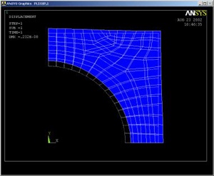
Main Menu > General Postproc > Plot Results > Deformed Shape
Select Def + undeformed and click OK.
This plots the deformed and undeformed shapes in the Graphics window. The maximum deformation DMX is 0.232E-08m as reported in the Graphics window. Note that the deformation is magnified in the plot so as to be visible.
The deformation would be better visible if the foreground and background were not of the same color. Turn off the background:
Utility Menu > PlotCtrls > Style > Background > Display Picture Background
To get the background back, you just have to select this again.
Animate the deformation:
Utility Menu > PlotCtrls > Animate > Deformed Shape...
Select Def + undeformed and click OK. Select Forward Only in the Animation Controller.
The left and bottom edges move parallel to themselves which means that the full deformed plate is also symmetric about these edges. This shows that the symmetry boundary condition at these edges is imposed correctly. The circular edge of the hole moves outward which is what one would expect from the outward pressure acting along it. Thus, the deformation of the structure agrees with the applied boundary conditions and matches with what one would expect from intuition.
Close the Animation Controller.
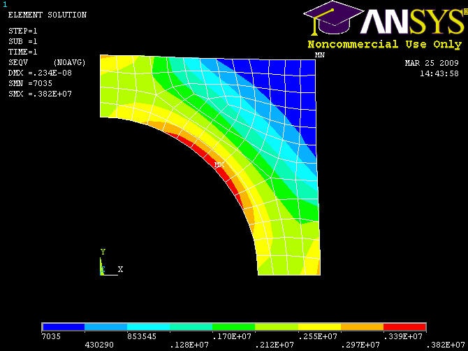
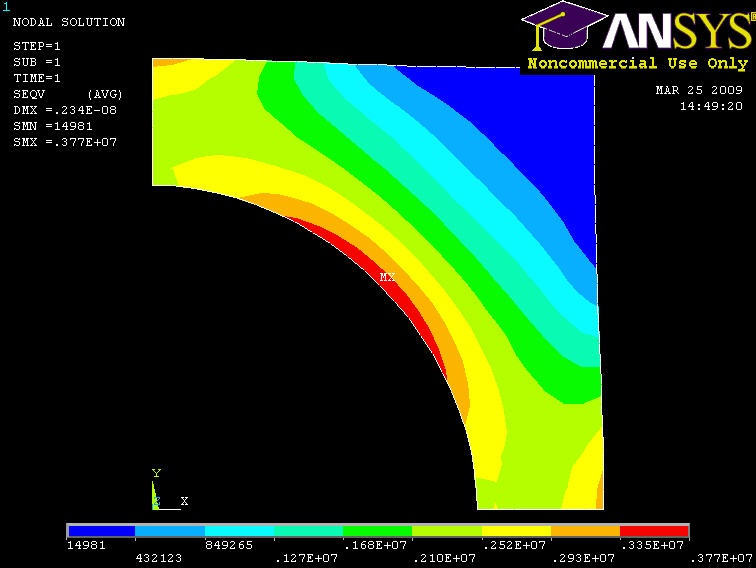
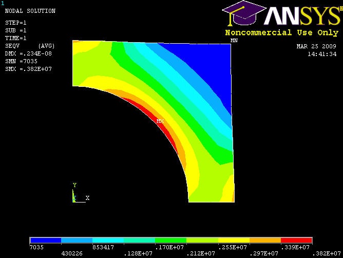
Plot Nodal Solution of von Mises Stress
To display the von Mises stress distribution as continuous contours, select
Main Menu > General Postproc > Plot results > Contour Plot > Nodal Solu
Select Nodal Solution > Stress > von Mises stress and click OK.

The contour plot will show you the locations of the maximum and minimum values with the labels MX and MN, respectively. Are these locations where you expect them? SMX and SMN values reported in the Graphics window are the corresponding maximum and minimum stress values.
The diagonal is an additional line of symmetry. How symmetric is your result about the diagonal?
Save this plot to a file:
Utility Menu > PlotCtrls > Hard Copy > To File
Select the file format you want and type in a filename of your choice under Save to: and click OK. Check that the file has been created in your working directory.
When you plot the "Nodal Solution", ANSYS obtains a continuous distribution as follows:
1. It determines the average at each node of the values of all elements connected to the node.
2. Within each element, it linearly interpolates the average nodal value obtained in the previous step.
Plot Element Solution of von Mises Stress
To obtain results without nodal averaging, select
Main Menu > General Postproc > Plot results > Contour Plot > Element Solu
Select Element Solution > Stress > von Mises stress and click OK. This displays the von Mises stress results as discontinuous element contours.
Save this plot to a file: Utility Menu > PlotCtrls > Hard Copy > To File
Element solution contours are determined by linear interpolation within each element but no nodal averaging is performed. The discontinuity between contours of adjacent elements is an indication of the gradient across elements. The inter-element discontinuities in our solution are relatively small compared to the stress levels. This indicates that the mesh resolution is reasonably good.
Query Results
To determine the value of the first principal stress σ1 at a selected location, select
Main Menu > General Postproc > Query Results > Subgrid Solu
This brings up the Query Subgrid Solution Data menu. Select Stress from the left list, 1st principal S1 from the right list and click OK.
This brings up the pick menu. You can click on any location in the geometry and ANSYS will print the σ1 value at that location. Try querying the values at a few locations. Note that the coordinates of the picked location and the corresponding solution value are reported in the pick menu.
Cancel the pick menu.
Go to Step 9: Validate the results
Step 9: Validate the results
It is very important that you take the time to check the validity of your solution. This section leads you through some of the steps you can take to validate your solution.
Simple Checks
Does the deformed shape look reasonable and agree with the applied boundary conditions? We checked this in step 8.
Do the reactions at the supports balance the applied forces for static equilibrium? To check this, select
Main Menu > General Postproc > List Results > Reaction Solu
Select All struc forc F for Item to be listed and click OK.
The total reaction force in the x-direction is -7000 N.
Applied force = (pressure) x (projected distance in x-direction of the line along which the constant pressure acts) = (p) (r) = 7000 N in positive x-direction.
So the reaction cancels out the applied force in the x-direction. Similarly, you can check that this is true in the y-direction also.
Refine Mesh
Let's repeat the calculations on a mesh with overall element size level under SmartSize set to 4 instead of 5 and compare the results on the two meshes. Delete the current mesh:
Main Menu > Preprocessor > Meshing > Mesh Tool
Select Clear under Mesh: and Pick All in the pick menu. The mesh is deleted.
Set the overall element size level under SmartSize to 4 by dragging the slider to the left. Click on Mesh and Pick All.
In the Output window, check how many elements are contained in this mesh? Your new mesh should have 320 quadrilateral elements.
Obtain a new solution: Main Menu > Solution > Solve > Current LS
Plot nodal solution of the von Mises stress:
Main Menu > General Postproc > Plot results > Contour Plot > Nodal Solu
Select Nodal Solution > Stress > von Mises stress and click OK
Compare this with the von Mises contours for the previous mesh:

The two results compare well with the finer mesh contours being smoother as expected. Compare the maximum stress and displacement values:
. |
Coarser Mesh |
Finer Mesh |
DMX |
0.232e-8m |
0.234e-8m |
SMX |
3.64MPa |
3.77MPa |
The maximum displacement value changes by less than 1% and the maximum von Mises stress value by less than 3%. This indicates that the meshes used provide adequate resolution.
Exit ANSYS
Utility Menu > File > Exit
Select Save Everything and click OK.
Reference
Cook, R.D., Malkus, D.S., Plesha, M.E., and Witt, R.J., Concepts and Applications of Finite Element Analysis, Fourth Edition, John Wiley and Sons, Inc., 2002.
Problem Set 1
Problem Statement
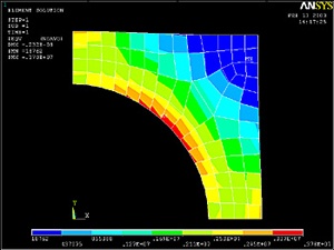
We used a 4-node quad element (PLANE42) in the tutorial. ANSYS also offers a 8-node quad element (PLANE82). Re-solve the tutorial problem using the PLANE82 element. Compare plots of the nodal and element solution of the von Mises stress for the two cases. You may use either mesh for this problem (although the final results presented here are done using the coarser mesh).
Hints
Look at the steps and think about which ones you have to change.
When you remesh the object, notice the following changes:

The number of nodes has increased!
To see why, do:
Utility Menu > PlotCtrls > Multi-plot Ctrls ...
Click OK. Then on the Multi-Plotting Window that comes up, deselect everything but Nodes and Elements.
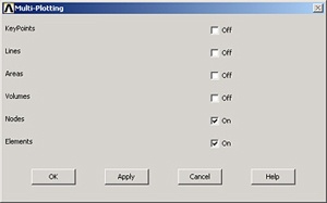
Click OK.
Then go to Plot > Multi-Plots
In the Graphics Window, you will now see the nodes in between the lines. There are 8 points for each quadrilateral area instead of the four we had before!

Final Result
Here are the Nodal and Element Solutions you should have gotten:
Nodal Solution

Element Solution