FLUENT - Flat Plate Boundary Layer - Setup (Physics)

Step 4: Setup (Physics)

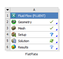
Your current Workbench Project Page should look comparable to the following image. Regardless of whether you downloaded the mesh and geometry files or if you created them yourself, you should have checkmarks to the right of Geometry and Mesh.



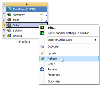
Next, the mesh and geometry data need to be read into FLUENT. To read in the data (Right Click) Setup > Refresh in the Workbench Project Page as shown in the image below.



After you click Update, a question mark should appear to the right of the Setup cell. This indicates that the Setup process has not yet been completed.

Launch Fluent

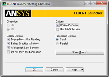
Double click on Setup in the Workbench Project Page which will bring up the FLUENT Launcher. When the FLUENT Launcher appears change the options to "Double Precision", and then click OK as shown below.The Double Precision option is used to select the double-precision solver. In the double-precision solver, each floating point number is represented using 64 bits in contrast to the single-precision solver which uses 32 bits. The extra bits increase not only the precision, but also the range of magnitudes that can be represented. The downside of using double precision is that it requires more memory.

Twiddle your thumbs a bit while the FLUENT interface starts up. This is where we'll specify the governing equations and boundary conditions for our boundary-value problem. On the left-hand side of the FLUENT interface, we see various items listed under Problem Setup. We will work from top to bottom of the Problem Setup items to setup the physics of our boundary-value problem. On the right hand side, we have the Graphics pane and, below that, the Command pane.

Check and Display Mesh

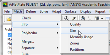
First, the mesh will be checked to verify that it has been properly imported from Workbench. In order to obtain the statistics about the mesh (Click) Mesh > Info > Size, as shown in the image below.



Then, you should obtain the following output in the Command pane.



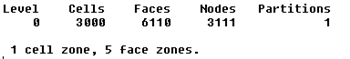
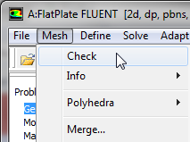
The mesh that was created earlier has 3,000 elements(50 x 60). Note that in FLUENT elements are called cells. The output states that there are 3,000 cells, which is a good sign. Next, FLUENT will be asked to check the mesh for errors. In order to carry out the mesh checking procedure (Click) Mesh > Check as shown in the image below.



You should see no errors in the Command Pane.

Problem Setup > General > Mesh > Display

Define Governing Equations

Problem Setup > Models > Energy

Use the default and click OK.

Problem Setup > Models > Viscous

Select Laminar under Model and click Edit.

 
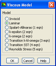
We want to leave the default value so you can click Cancel.

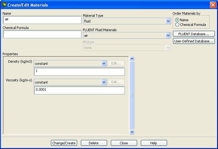
Problem Setup > Materials

Double click air or select it and click Create/Edit. Make sure air is selected under Fluid Materials. Set Density to 1.00 and Viscosity to 1e-4 so that we can get Re of 1e4.

Higher Resolution Image
Click Change/Create.

Define Boundary conditions

Problem Setup > Boundary Conditions

Set the inlet boundary type to velocity-inlet. Then click Set...Set the velocity magnitude to 1 m/s. Set the outlet type to pressure-outlet boundary. Use gauge pressure of 0 Pa.Use the default value of wall for the center line. Set the far field to symmetry boundary type. Symmetry boundary condition means that the component normal to the wall is zero.

Problem Setup > Boundary Conditions

 > Operating Conditions

 
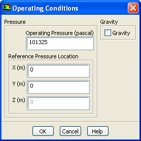
Use the default value. Click OK.

Go to Step 5: Solution