Page History

Step 4: Setup (Physics)

If you have skipped the previous mesh generation steps 1-3, you can download the mesh by right-clicking on this link. Save the file as nozzle.msh in your working directory. You can then proceed with the flow solution steps below.

Launch FLUENT

Start > Programs > ANSYS 12.0 > Fluid Dynamics > FLUENT

Select 2D from the list of options and click OK.

Import File

Main Menu > File > Read > Case...

Navigate to your working directory and select the nozzle.msh file. Click OK.

The following should appear in the FLUENT window:

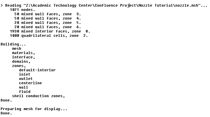
Check that the displayed information is consistent with our expectations of the nozzle mesh.

Check and Display Mesh

First, we check the grid to make sure that there are no errors.

Under Problem Setup > General > Mesh > Check (button)

Any errors in the grid would be reported at this time. Check the output and make sure that there are no errors reported.

Main Menu > Mesh > Info > Size

How many cells and nodes does the grid have?

The mesh is being displayed by default but the steps to accomplish this when the grid is not being displayed are the following:

Main Menu > Display > Mesh

Make sure all items under Surfaces is selected. Then click Display. The graphics window opens and the mesh is displayed in it.

Some of the operations available in the graphics window are:

Translation: The mesh can be translated in any direction by holding down the Left Mouse Button and then moving the mouse in the desired direction.

Zoom In: Hold down the Middle Mouse Button and drag a box from the Upper Left Hand Corner to the Lower Right Hand Corner over the area you want to zoom in on.

Zoom Out: Hold down the Middle Mouse Button and drag a box anywhere from the Lower Right Hand Corner to the Upper Left Hand Corner.

The mesh has 50 divisions in the axial direction and 20 divisions in the radial direction. The total number of cells is 50x20=1000. Since we are assuming inviscid flow, we won't be resolving the viscous boundary layer adjacent to the wall. (The effect of the boundary layer is small in our case and can be neglected.) Thus, we don't need to cluster nodes towards the wall. So the mesh has uniform spacing in the radial direction. We also use uniform spacing in the axial direction.

Look at specific parts of the mesh by choosing each boundary (centerline, inlet, etc) listed under Surfaces in the Mesh Display menu. Click to select and click again to deselect a specific boundary. Click Display after you have selected your boundaries.

Define Solver Properties

Define > Models > Solver...

We see that FLUENT offers two methods ("solvers") for solving the governing equations: Pressure-Based and Density-Based. To figure out the basic difference between these two solvers, let's turn to the documentation.

Main Menu > Help > User's Guide Contents ...

This should bring up FLUENT 12.0 User's Guide in your web browser. If not, access the User's Guide from the Start menu: Start > Programs > ANSYS 12.0 > Help > FLUENT Help. This will bring up the FLUENT documentation in your browser. Click on the link to the user's guide.

Go to chapter 26 in the user's guide. It discusses the Pressure-Based and Density-Based solvers. Section 26.1 introduces the two solvers:

" In ANSYS FLUENT, two solver technologies are available:

• pressure-based
• density-based

Both solvers can be used for a broad range of flows, but in some cases one formulation may perform better (i.e., yield a solution more quickly or resolve certain flow features better) than the other. The pressure-based and density-based approaches differ in the way that the continuity, momentum, and (where appropriate) energy and species equations are solved, as described in this section in the separate +Theory Guide.+The pressure-based solver traditionally has been used for incompressible and mildly compressible flows. The density-based approach, on the other hand, was originally designed for high-speed compressible flows. Both approaches are now applicable to a broad range of flows (from incompressible to highly compressible), but the origins of the density-based formulation may give it an accuracy (i.e. shock resolution) advantage over the pressure-based solver for high-speed compressible flows."

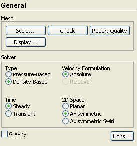
Since we are solving a high-speed compressible flow, let's pick the density-based solver.

In the Solver menu, select Density Based.

Under Space, choose Axisymmetric. This will solve the axisymmetric form of the governing equations.

Then we will setup the models for the problem:

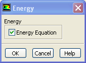
Define > Models > Energy > Edit

The energy equation needs to be turned on since this is a compressible flow where the energy equation is coupled to the continuity and momentum equations.

Make sure there is a check box next to Energy Equation and click OK.

Define > Models > Viscous - Laminar > Edit

Select Inviscid under Model.

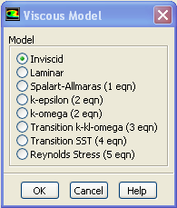
Click OK.

This means the solver will neglect the viscous terms in the governing equations.

Define > Materials

Select air under Fluid materials and click the Create/Edit... button. Under Properties, choose Ideal Gas next to Density. You should see the window expand. This means FLUENT uses the ideal gas equation of state to relate density to the static pressure and temperature.

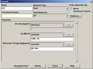
Click Change/Create. Close the window.

Define > Operating Conditions

We'll work in terms of absolute rather than gauge pressures in this example. So set Operating Pressure in the Pressure box to 0.

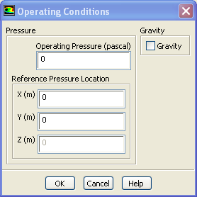
Click OK.

It is important that you set the operating pressure correctly in compressible flow calculations since FLUENT uses it to compute the absolute pressure used in the ideal gas law.

Define > Boundary Conditions

Set boundary conditions for the following surfaces: inlet, outlet, centerline, wall.

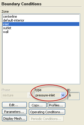
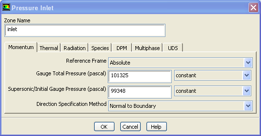
Select inlet under Zone and pick pressure-inlet under Type as its boundary condition. Automatically, the Pressure Inlet window should come up.

Set the total pressure (noted as Gauge Total Pressure in FLUENT) at the inlet to 101,325 Pa as specified in the problem statement. For a subsonic inlet, Supersonic/Initial Gauge Pressure is the initial guess value for the static pressure. This initial guess value can be calculated from the 1D analysis since we know the area ratio at the inlet. This value is 99,348 Pa. Note that this value will be updated by the code. After you have entered the values check that under the Thermal tab, the Total Temperature is 300K. Then click OK to close the window.

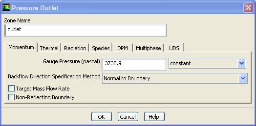
Using the same steps as above, pick pressure-outlet as the boundary condition for the outlet surface. Then, when the Pressure Outlet window comes up, set the pressure to 3738.9 as specified in the problem statement. Click OK.

Set the centerline zone to axis boundary type. Accept any prompts that might appear and leave the name as centerline if you'd like.

Make sure that wall zone is set to wall boundary type.

Go to Step 5: Solution

See and rate the complete Learning Module

Go to all FLUENT Learning Modules