 Sign-up for free online course on ANSYS simulations!
...
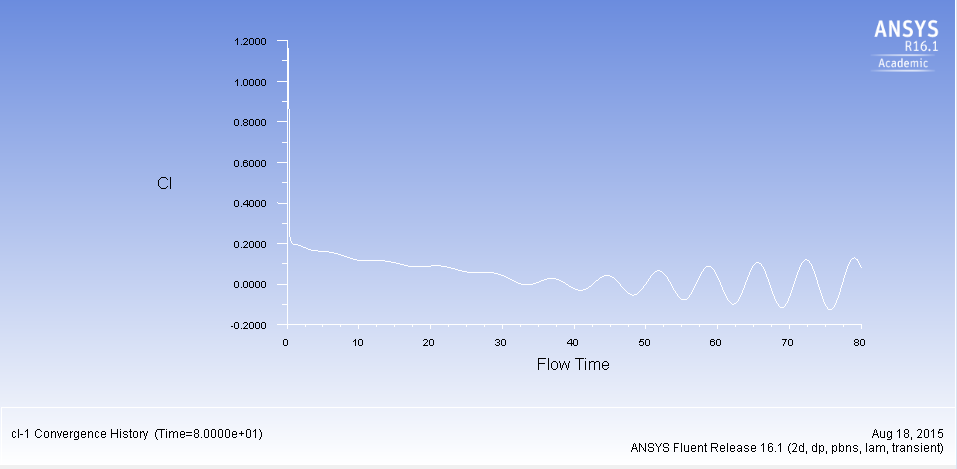
Above, we see the variation of the lift coefficient with the flow time if we had not patched the region.
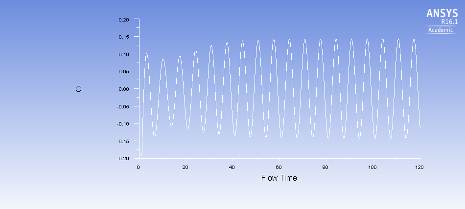
Above, we see the variation of the lift coefficient with the folw time with the region patch. This patch was using .5 < x < 32 and 0 < y < 32. Note how we see the shedding more quickly than if we had not patched the region.
...
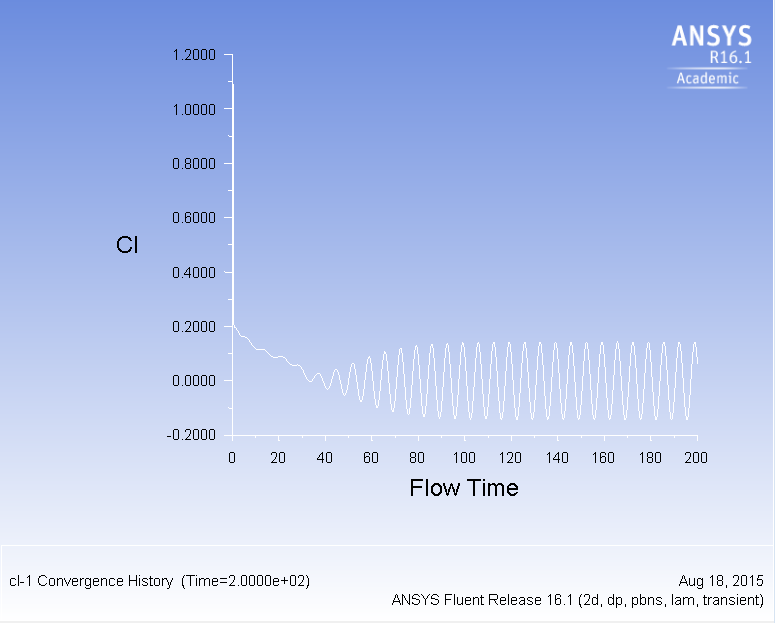
In order to effectively capture the vortex shedding, a small enough timestep was needed. It was recommeded to have roughly 20 - 25 timesteps per cycle hence we used a timestep of .2. The resulting plot in the numerical results showing how the lift coefficient oscillated due to the vortex shedding is shown below. To compare the effect of the timestep size, we continue to plot the lift coefficient after the oscillations have been established with a timestep of .02 seconds. Changing the timestep changes the resolution, so with a smaller timestep we expect a better resolution when seeing the oscillation of the lift coefficient.
Timestep = .2 s
...
The Strouhal Number from the literature is reported to be .183. It is expected that the Strouhal Number will be roughly .2 for flow past the cylinder. By plotting for 600 more time steps, we obtain the Cl vs. Flow time graph below and see how the shedding has become constant. We can do a rough estimate of the frequency by taking an amount of time and seeing how many peaks occur in that time. Using this frequency, we can calculate the Strouhal Number for our simulation.
We see about 10 peaks in 60 seconds, giving a frequency of .1667 which is close to the literature and around what we would expect.
...