Page History

...

Solution Methods

Click on Solution Methods then click on Momentum and select Bounded Central Differencing as shown in the image below. Also choose, Second order for Pressure and Second Order Implicit under Transient Formulation.  as

Click Here for Higher Resolution

...

Here, the flow field will be initialized to the values at the inlet. In order to carry out the initialization click on Solution Initialization then click on Compute from and select inlet as shown below. 

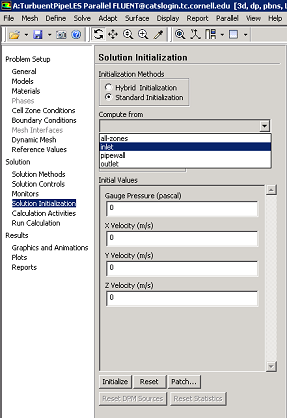
Click Here for Higher Resolution

Then click initialize to initialize the domain with an initial guess. This completes the initialization.

...

FLUENT reports a residual for each governing equation being solved. The residual is a measure of how well the current solution satisfies the discrete form of each governing equation. We'll iterate the solution until the residual for each equation falls below 1e-6. In order to specify the residual criteria (Click) Monitors > Residuals > Edit..., as shown in the image below. 

...

Next, change the residual under Convergence Criterion for continuity, x-velocity,and y-velocity, all to 1e-6, as can be seen below.

...

Click Here for Higher Resolution

Lastly, click OK to close the Residual Monitors menu.

Execute Calculation

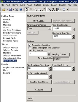
Note that, we have to run the transient simulation to a statistically stationary state and then collect statistics. Click on Run Calculation then choose the Time Step Size(s) as 1e-05 and the Number of Time Steps  as 20000. Also choose Extrapolate Variables option (refer to FLUENT documentation for information) and leave the Max Iterations/Time Step as 20 (default). The corresponding image is shown below.

...

As a safeguard save the project now. Now, click on Calculate in order to run the calculation. The residuals for each iteration are printed out as well as plotted in the graphics window as they are calculated. The residuals decrease during the inner iterations and jump again when we advance by one time step as shown in image below.

...

In this simulation, it is verified that the statistically stationary state is reached by advancing the simulation from 0s to 0.1s in physical time i.e. using only 10,000 time steps with 1e-05s time step size with 20 inner iterations.When statistically stationary state is reached, statistics have to be collected by advancing the physical time from 0.1s to atleast 0.15s. Use 5,000 time steps with 1e-05 time step size with 20 inner iterations. This is done as shown in the figure below. Select the Data Sampling for Time Statistics to start collecting the statistics. You will see the physical time for which the statistics have been collected across Time Sampled (s). 

Click Here for Higher Resolution

...