Numerical Results

...

Okay! Now let's look at the numerical solution to the boundary value problem as calculated by ANSYS. Let's start by examining how the plate deformed under the load. Before you start, make sure the software is working in the same units you are by looking to the menu bar and selecting Units > US Customary (in, lbm, lbf, F, s, V, A). Also, select the pan tool by clicking the pan button from the top bar. This will allow you to zoom by scrolling the mouse wheel, and move the image by left-clicking and dragging.

...

Now, look at the Outline window, and select Solution > Total Deformation. First, we will look at just the deformation of the plate, without contours. To do this, select the Contours button, , and select Solid Fill.

There are a few things we can determine from this picture. Let's use our intuition and the work we did in the pre-analysis to compare to the result ANSYS gives us. First, let's look at the bottom and left edges of the plate. We can see that the deformation on these edges is parallel to the sides, which agrees with the symmetry boundary condition. The top edge of the plate has deformed downwards, which is due to the effects of Poisson's ratio. The right edge has moved to the right, which is consistent with the expected behavior, due to the plate being in tension. So we can deduce the following boundary conditions from looking at the deformation.

...

Animate the deformation by pressing Play in the Animation tool bar along the bottom of the screen. This linearly interpolates between the initial and final deformed state.

...

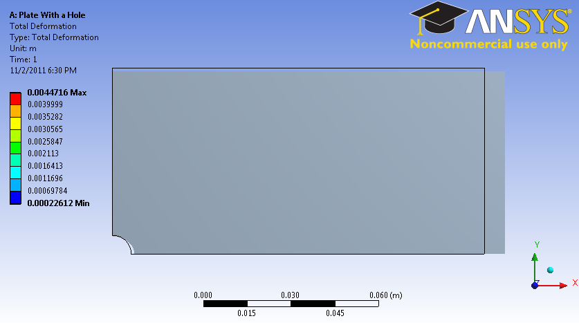
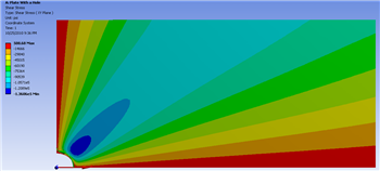
To get back the color contours of deformation values, select the Contours button and choose Contour Bands. The colored section refers to the magnitude of the deformation (in inches) while the black outline is the undeformed geometry superimposed over the deformed model. The more red a section is, the more it has deformed while the more blue a section is, the less it has deformed. Notice that far from the hole, the deformation is linearly varying, similar to a bar in tension. Now let's look at the value of the largest deformation. Looking at the top of the color bar, we see that the largest deformation is 0.176 inches. From our pre-analysis, we estimated that the deformation was ~ 0.17 inches - a 2% difference. This is one check on our ANSYS result.

...

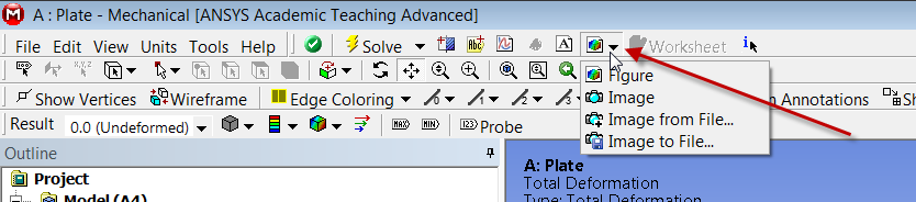
You can save the image to a file using the Image to File option shown below.

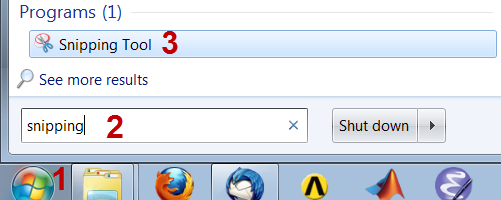
Sometimes, you get an error saying "The display settings are Windows Aero and image capture might not work." In that case, you can use the Windows 7 snipping tool which can be accessed from the Start > Programs menu as shown below.

Draw a rectangle around the screen area that you want to capture and save to an image file.

...

Now let's look at the radial stresses in the plate. Look to the outline window and click Solution > Sigma-r. This will display the radial stresses.

...

Now, let's compare the simulation to our pre-calculations for the theta stress. Look to the Outline window, then click Solution > Sigma-theta

First, let's compare the case when r = a. From the pre-analysis, we found that the stress at the hole acts as a function of theta. Specifically:

...

Now let's look at how the simulation match our predictions for the shear stress. Look to the Outline window, then click Solution > Tau-r-theta

In our pre-analysis, we determined that at r = a the shear stress should be 0 psi. Using our probe tool, we find that the stress ranges between -5 and -500 psi at the hole. Because 500 psi is .05% of the average stress, we can say this result does represent what we expect to happen very well.

...

Now lets examine the stress in the x-direction. Look to the Outline window, then click Solution > Sigma-x

From this, you can see that most of the plate is in constant stress, and there is a stress concentration around the hole. The more red areas correspond to a high, tensile (positive) stress and the bluer areas correspond to areas of compressive (negative) stress. Let's use the probe tool to compare the ANSYS simulation to what we expected from calculation. In the menu bar, click the Probe button; this will display the Sigma-x values at the cursor location as you hover over the plate.

...

Add a normal stress object under Solution in the tree: Stress > Normal. Change the scoping method to Path and select left edge for Path.

...