Physics Setup

Regardless of whether you downloaded the mesh and geometry files or if you created them yourself, you should have checkmarks to the right of Geometry and Mesh. Your current Workbench Project Page should look comparable to the following image.

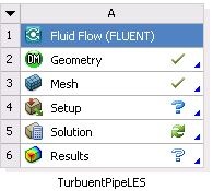
A question mark should appear to the right of the Setup cell. This indicates that the Setup process has not yet been completed. This means that the mesh and the geometry data need to be read into FLUENT.

Launch Fluent

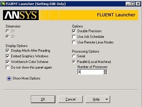
Double click on Setup in the Workbench Project Page which will bring up the FLUENT Launcher. When the FLUENT Launcher appears change the Options to "Double Precision", and Processing Options to "Parallel (Local Machine)" with Number of Processes equal to "4" or to the available number of processors at your end. Click OK as shown below.

Higher Resolution Image

Twiddle your thumbs a bit while the FLUENT interface starts up. This is where we'll specify the governing equations and boundary conditions for our problem. On the left-hand side of the FLUENT interface, we see various items listed under Problem Setup. and Solution. We will work from top to bottom of both these items to setup the physics of our boundary-value problem. On the right hand side, we have the Graphics pane and, below that, the Command pane.

Check and Display Mesh

First, the mesh will be checked to verify that it has been properly imported from Workbench. (Click) Mesh > Check and make sure that the minimum volume is positive. It is a good practice to check if x/y/z - domain extents are according to the dimensions given in the problem specification.

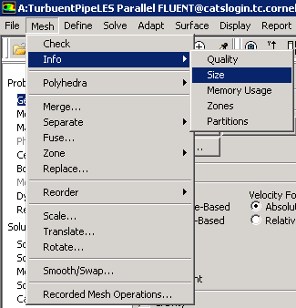
In order to obtain the statistics about the mesh (Click) Mesh > Info > Size, as shown in the image below.

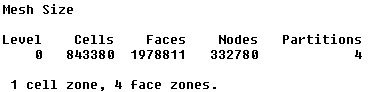
Then, you should obtain the following output in the Command pane.

In order to bring up the display options (Click) General > Mesh > Display. Make sure you have inlet, outlet, pipewall and interior-solid in Surfaces as shown in the figure below.

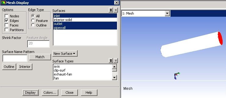
Please review the "Laminar Pipe Flow" tutorial to understand how to rotate, zoom-in and zoom-out the geometry in the Graphics Window.

Define Solver Properties

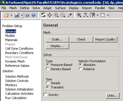
In this section the various solver properties will be specified in order to obtain the proper solution. On the left side of the window (Click) Problem Setup> General. Make sure that Pressure-Based is selected under Type and Transient is selected under Time in the Solver section. Note: LES is a transient simulation where the solution is marched in time.

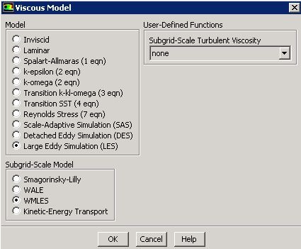
Next, the Viscous Model parameters will be specified. In order to open the Viscous Model Options (Click) Problem Setup > Models > Viscous - Laminar > Edit.... Click Large Eddy Simulation under Model and WMLES under Subgrid-Scale Model. Click OK.

An Information box will appear as shown below, click OK. Basically, FLUENT switches the discretization scheme for momentum equation to Bounded Central-Differencing. It also urges to change the order to Second Order Implicit for Transient Formulation in the Solution Methods, which we will do in the later stages.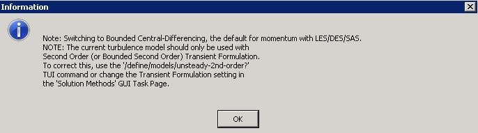

For incompressible flows, the energy equation is decoupled from the continuity and the momentum equations. So the energy equation is not solved. Make sure that Energy is set to Off in Problem Setup > Models > Energy.

Define Material Properties

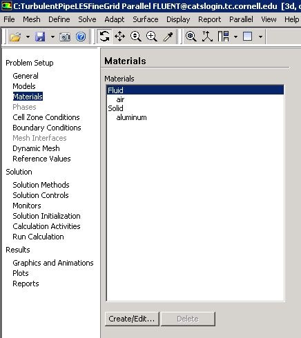
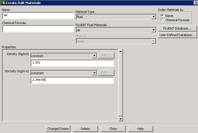
Now, the properties of the fluid that is being modeled will be specified. The properties of the fluid were specified in the Problem Specification section. In order to create a new fluid (Click) Problem Setup > Materials > Fluid > Create/Edit... as shown in the image below.

In the Create/Edit Materials menu set the Density to 1.331 kg/m^3 (constant) and set the Viscosity to 2.34e-05 kg/(ms) (constant) as shown in the image below.

Higher Resolution Image

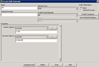
Click Change/Create. Close the window.

Define Boundary Conditions

At this point the boundary conditions for the three Named Selections will be specified.

Inlet Boundary Condition

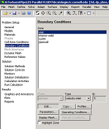
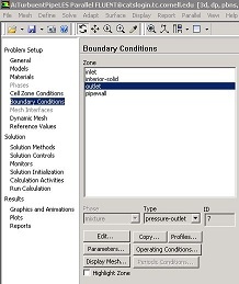
In order to start the process (Click) Problem Setup > Boundary Conditions > inlet > Edit... as shown in the following image.

Inlet_BC.png

Higher resolution Image

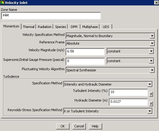
Note that the Boundary Condition Type should have been automatically set to velocity-inlet. Now, the velocity at the inlet will be specified. In the Velocity Inlet menu set the Velocity Specification Method to Magnitude, Normal to Boundary, set the Velocity Magnitude (m/s) to 6.58 m/s and set the Fluctuation Velocity Algorithm to Spectral Synthesizer (this is needed to fluctuate the velocity at the inlet). Also set the Turbulence Specification Method to Intensity and Hydraulic Diameter. Set the value of Turbulent Intensity (%) to 10 % and Hydraulic Diameter (m) to 0.0127 m. Finally set the Reynolds-Stress Specification Method to K or Turbulent Intensity as shown below. Click OK to close the Velocity Inlet menu.

Outlet Boundary Condition

First, select outlet in the Boundary Conditions menu, as shown below.

Higher Resolution Image

As can be seen in the image above the Type should have been automatically set to pressure-outlet. If the Type is not set to pressure-outlet, then set it to pressure-outlet. Now, no further changes are needed for the outlet boundary condition.

Pipe Wall Boundary Condition

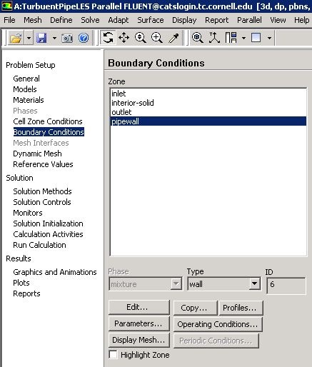
First, select pipewall in the Boundary Conditions menu, as shown below. 

Higher Resolution Image

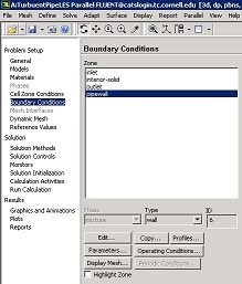
As can be seen in the image above the Type should have been automatically set to wall. If the Type is not set to wall, then set it to wall. Now, no further changes are needed for the pipe_wall boundary condition. Also make sure that the boundary condition Type for interior-solid is Interior.

It is a good practice to change the Reference Values now, these values can be useful when we are postprocessing results later on. (Click)Problem Setup > Reference Values. Select Compute from as inlet.

Save

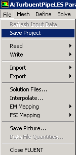
In order to save your work (Click)File > Save Project as shown in the image below.

Go to Step 5: Numerical Solution

Go to all FLUENT Learning Modules