 Sign-up for free online course on ANSYS simulations!
Authors: Yong Wang & Said Elghobashi, UC Irvine
Problem Specification
1. Pre-Analysis & Start-Up
2. Geometry
3. Mesh
4. Physics Setup
5. Numerical Solution
6. Numerical Results
7. Verification & Validation
Exercises
Comments
Numerical Results
The results steps shown below are for the CFD-Post postprocessor that is included in ANSYS Workbench.
Velocity Vectors
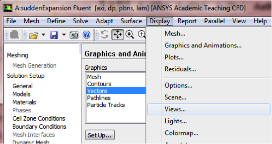
One can plot vectors in the entire domain, or on selected surfaces. Let us plot the velocity vectors for the entire domain to see how the flow develops downstream from the inlet and redevelops from the expansion entrance. First, click on Graphics & Animations. Next, double click on Vectors which is located under Graphics. Then, click on Display. Zoom into the region near the inlet. The length and color of the arrows represent the velocity magnitude. The vector display is more intelligible if one makes the arrows shorter as follows:
Change Scale to 0.4 in the Vectors menu and click Display.
The laminar pipe flow was modeled asymmetrically; however, the plot can be reflected about the axial axis to get an expanded sectional view. In order to carry this out (Click) Display > Views... as shown below.
Under Mirror Planes, only the axis (or centerline) surface is listed since that is the only symmetry boundary in the present case. Select axis (or centerline) and click Apply, as shown below.
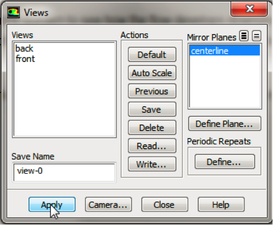
Then click Close to exit the Views menu. Your vector field should have been reflected across the axially axis as, shown below.
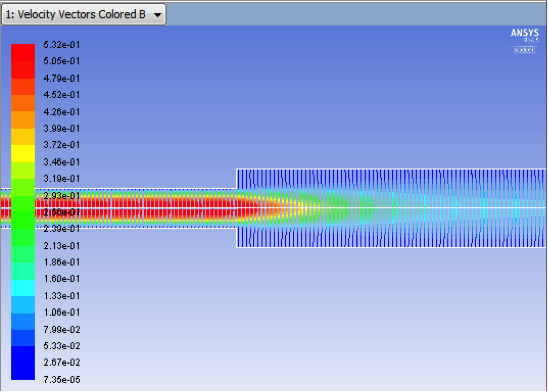
The velocity vectors provide a picture of how the flow develops downstream from the inlet and redevelops from the expansion entrance.
Centerline Velocity
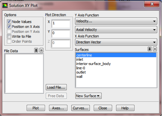
Here, we'll plot the variation of the axial velocity along the centerline. In order to start the process (Click) Results > Plots > XY Plot... > Set Up.. as shown below
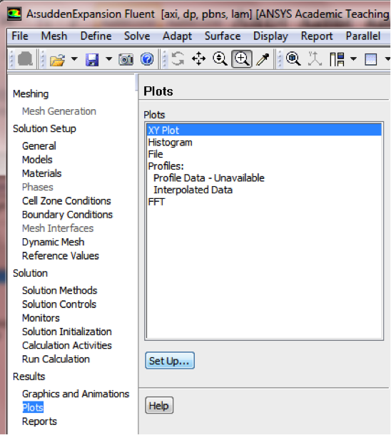
In the Solution XY Plot menu make sure that Position on X Axis is selected, and X is set to 1 and Y is set to 0. This tells FLUENT to plot the x-coordinate value on the abscissa of the graph. Next, select Velocity... for the first box underneath Y Axis Function and select Axial Velocity for the second box. Please note that X Axis Function and Y Axis Function describe the x and y axes of the graph, which should not be confused with the x and y directions of the pipe. Finally, select centerline under Surfaces since we are plotting the axial velocity along the centerline. This finishes setting up the plotting parameters. Your Solution XY Plot should look exactly the same as the following image.
Now, click Plot. The plot of the axial velocity as a function of distance along the centerline now appears.
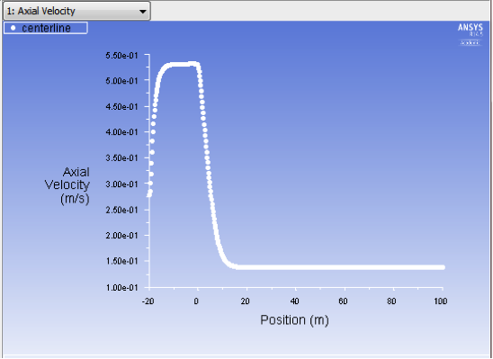
In the graph that comes up, we can see that the velocity reaches a constant value (about 5.25e-1 m/s) beyond a certain distance from the inlet. This is the fully-developed flow region in the small pipe. When the flow pass the expansion entrance at x=0 m, the velocity will decrease due to the sudden expansion of the pipe. After another development, the velocity will reach a constant value (about 1.5e-1m/s) again.
Saving the Plot
In this section, we will save the data from the plot and a picture of the plot. The data from the plot will be saved first. In order to save the plot data open the Solution XY Plot menu and then select Write to File, which is located under Options. The Plot button should have changed to Write.... Click on Write..., and then enter vel.xy as the XY File Name. Next, click OK. Check that this file has been created in your FLUENT working directory. Lastly, close the Solution XY Plot menu.
At this point, we'll save a picture of the plot. First click on File then click Save Picture, as shown below.
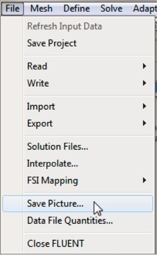
Under Format, choose one of the following three options: EPS, TIFF, or JPG. After selecting your desired image format and associated options, click on Save... Enter vel.eps, vel.tif, or vel.jpg depending on your format choice and click OK. Verify that the image file has been created in your working directory. You can now copy this file onto a disk or print it out for your records.