Numerical Results

Displacement

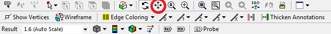
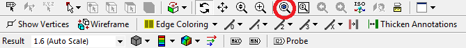
Okay! Now let's look at the numerical solution to the boundary value problem as calculated by ANSYS. Let's start by examining how the plate deformed under the load. Before you start, make sure the software is working in the same units you are by looking to the menu bar and selecting Units > US Customary (in, lbm, lbf, F, s, V, A). Also, select the pan tool by clicking the pan button from the top bar. This will allow you to zoom by scrolling the mouse wheel, and move the image by left-clicking and dragging.

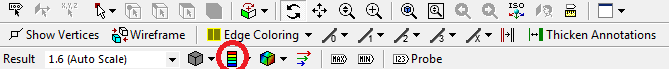
Now, look at the Outline window, and select Solution > Total Deformation. First, we will look at just the deformation of the plate, without contours. To do this, select the Contours button, , and select Solid Fill. To display an undeformed body, click the Result drop-down menu next to the Contours button, and select Undeformed. 

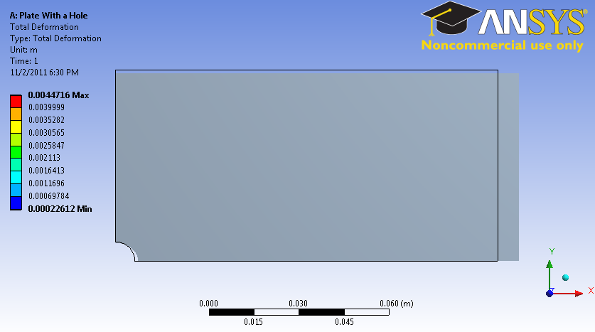
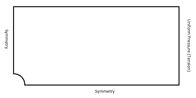
There are a few things we can determine from this picture. Let's use our intuition and the work we did in the pre-analysis to compare to the result ANSYS gives us. First, let's look at the bottom and left edges of the plate. We can see that the deformation on these edges is parallel to the sides, which agrees with the symmetry boundary condition. The top edge of the plate has deformed downwards, which is due to the effects of Poisson's ratio. The right edge has moved to the right, which is consistent with the expected behavior, due to the plate being in tension. So we can deduce the following boundary conditions from looking at the deformation.

Animate the deformation by pressing Play in the Animation tool bar along the bottom of the screen. This linearly interpolates between the initial and final deformed state.

To get back the color contours of deformation values, select the Contours button and choose Contour Bands. The colored section refers to the magnitude of the deformation (in inches) while the black outline is the undeformed geometry superimposed over the deformed model. The more red a section is, the more it has deformed while the more blue a section is, the less it has deformed. Notice that far from the hole, the deformation is linearly varying, similar to a bar in tension. Now let's look at the value of the largest deformation. Looking at the top of the color bar, we see that the largest deformation is 0.17605 inches. From our pre-analysis, we found that the deformation was 0.1724 inches - a 2% difference. Being that our calculation was only an estimate (we neglected the hole), this seems reasonable.

Sigma-r

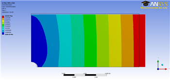
Now let's look at the radial stresses in the plate. Look to the outline window and click Solution > Sigma-r. This will display the radial stresses.

Does this match what we expect? First, let's examine the hole at r = a. From our pre-calculations, we found that the stress at the hole in the radial direction should be 0. Zooming in with the middle mouse wheel and using our probe tool, we find that the stress in this area ranges from -450 to 450 psi. Although the simulation does not approach exactly zero, keep in mind that 450 psi is less than 1% of the average stress, so it can be thought of as approximately zero. Also, we expect this value to get closer to zero as we refine the mesh.

In order to zoom out and view the whole solution, select the zoom to fit button from the toolbar.

Now, let's first look at the case when r >> a. As we found in the pre-calculations, when r >> a, the radial stress is a function of the angle theta only. This matches the behavior seen in the simulation. From our Pre-Calculations, we also found that . Using the probe tool, we find that indeed at this location, the stress is equal to 1e6 psi, which is the value we calculated in our Pre-Analysis. Also from our Pre-Analysis, we found that when .
Checking the simulation with our trusty probe tool, we find that the ANSYS simulation matches up quite nicely with our calculation.

Sigma-Theta

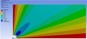
Now, let's compare the simulation to our pre-calculations for the theta stress. Look to the Outline window, then click Solution > Sigma-theta

First, let's compare the case when r = a. From the pre-analysis, we found that the stress at the hole acts as a function of theta. Specifically:

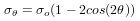
From this equation, we find that at zero degrees, we expect the stress to be -1e6 psi at zero degrees and at 90 degrees, we expect the stress to be 3e6 psi. Zoom in close to the hole to view the stresses there. From the simulation we find that the stress at 0 degrees is -1.0285e6 psi (a 3% deviation), and the stress at 90 degrees is 3.0323e6 psi (a 1 % deviation). The deviations are due to the infinite plate assumption in the theory.

Now, let's look at the case when r >> a. From our pre-calculations, we found that the theta stress is a function of theta only. This behavior is represented in the simulation. Also, for r >> a and the stress is equal to .
Using the probe tool and hovering over this area, we see that the stress is indeed equal to Sigma-o. However, looking at the area when , we find that the stress from the simulation is between 1000 psi and 2000 psi. Although this seems large compared to zero, one must keep in mind that the stress at this location is 1% of the average stress. We expect that the stress here will get closer to zero on refining the mesh since the numerical error becomes smaller.

Tau-r-theta

Now let's look at how the simulation match our predictions for the shear stress. Look to the Outline window, then click Solution > Tau-r-theta

In our pre-analysis, we determined that at r = a the shear stress should be 0 psi. Using our probe tool, we find that the stress ranges between -5 and -500 psi at the hole. Because 500 psi is .05% of the average stress, we can say this result does represent what we expect to happen very well.

In our pre-calculations, we determined that far from the hole the shear stress should be a function of theta only. This can be shown by using the probe tool a hovering over a radial line from the hole. The colors (representing higher and lower stresses) only change only as the angle changes, but not as the move away from the hole. We also found that far from the hole at the stress is zero

Using the probe tool, we can see that this is indeed the case for the simulation as well.

Sigma-x

Now lets examine the stress in the x-direction. Look to the Outline window, then click Solution > Sigma-x

From this, you can see that most of the plate is in constant stress, and there is a stress concentration around the hole. The more red areas correspond to a high, tensile (positive) stress and the bluer areas correspond to areas of compressive (negative) stress. Let's use the probe tool to compare the ANSYS simulation to what we expected from calculation. In the menu bar, click the Probe button; this will display the Sigma-x values at the cursor location as you hover over the plate.

Start by hovering over the area far from the hole. The stress is about 1e6 psi, which is the value we would expect for a plate in uniaxial tension. If you click the max tag (located adjacent to the probe tool in the menu bar), it will locate and display the maximum stress, which is shown as 3.0335e6 psi. This is about a 0.0055% difference from the calculation we did in the Pre-Analysis, which is a negligible difference.

Go to Step 3: Verification and Validation

Go to all ANSYS Learning Modules